Populations
Populations. Large populations. Terns. Small populations. Dryopteris fragrans , a rare cliff fern. Dynamic populations. Homo sapiens. Complex populations. Markers: isozymes. AFLPs. MMMMM. Illumina Beadstation genotyping for SNPs. High throughput genotypins Genotyping of a cross:

Populations
E N D
Presentation Transcript
Large populations Terns
Small populations Dryopteris fragrans, a rare cliff fern
Dynamic populations Homo sapiens
AFLPs MMMMM
IlluminaBeadstationgenotyping for SNPs • High throughput genotypins • Genotyping of a cross: • Low cost per genotype (5-20 cents) but need to assay for large number of genotypes (either 384, or 768, or 1586) makes total cost large (thousands of $)
What do populations have to do with genetic markers • Influence levels of diversity • Conversely, polymorphic genetic markers can infer many population processes • Emphasis in FRST432 is the latter
Quantifying genetic variation Gene frequency Genetic diversity Hardy-Weinberg
Estimation of gene frequency For co-dominant loci, simply count the numbers (“gene counting method”) Gene counting method also is the “maximum likelihood estimate”
Estimation of allele frequency MN blood group: genotype number MM 392 MN 707 NN 320 Total: 1419 (actual sample size is twice) Frequency of M=PM=(2 x 392 + 707)/[2 x 1419]=0.525 Frequency of N is 1-PM
Estimation of gene frequency Estimation based upon gene counting pA = (2NAA+NAa.)/(2NAA+2NAa+2Naa) More theoretical relationship pA = fAA+.5fAa F’s are frequencies Var(pA) = Var(pa) = pA (1-pA)/(2N) Binomial sampling variance Construct confidence interval
Hardy-Weinberg Predict genotypic frequencies from gene frequencies F(AA)=p2 F(Aa)=2pq F(aa)=q2 Expansion of (p+q)2 HW is basis for almost all models Inbreeding also detected as excess of homozygotes
Historical context Is the population going to be driven to a particular frequency for an allele simply because it is inherited in a Mendelian fashion? Is the recessive phenotype driven to occur in 25% of the population? Hardy and Weinberg proved this was false
HW “Equilibrium” Equilibrium = nothing changes across generations Genotypes are transient, broken up each generation Reconstituted randomly into zygotes Reached in just one generation
Assumptions of HW No directive forces No mutation, migration, selection No dispersive forces Infinite population size, random mating
Predictions of HW Allele frequencies unchanged over time After one generation, genotypic frequencies unchanged over time Allele frequencies, not genotypic frequencies, are sufficient parameters for models
The fundamental measure of genetic variation: expected heterozygosity At one locus, gene frequency for i-th allele is expected Hardy-Weinberg frequency of homozygous genotype is Over all possible alleles i, i=1,n, the probability that the locus is homozygous for any allele is
Expected heterozygosity = 1-expected homozygosity often referred to as gene diversity
Heterozygosity at 20 variable allozymes out of 71loci sampled in a population of European people Gene Locus Enzyme Encoded Heterozygosity H Aph Alkaline phosphatase (placental) 0.53 Acph Acid phosphatase 0.52 Gpt Glutamate-pyruvate transaminase 0.50 Adh-3 Alcohol dehydrogenase-3 0.48 Peps Pepsinogen 0.47 Pgm-2 Phosphoglucomutase-2 0.38 Pept-A Peptidase-A 0.37 Pgm-1 Phosphoglucomutase-l 0.36 Me Malic enzyme 0.30 Ace Acetylcholinesterase 0.23 Adn Adenosine deaminase 0.11 Gput Galactose-1-phosphate uridyl transferase 0.11 Adk Adenylate kinase 0.09 Amy Amylase (pancreatic) 0.09 Adh-2 Alcohol dehydrogenase-2 0.07 6Pgdh 6-Phosphogluconate dehydrogenase 0.05 Hk Hexokinase (white-cell) 0.05 Got Glutamate-oxaloacetate transaminase 0.03 Pept-C Peptidase-C 0.02 Pept-D Peptid ase-D 0.02 51 Loci invariant (Monomorphic) 0.00 After H. Harris and D. A. Hopkinson, J. Human Genetics
Variation of diversity among species Explaining levels of diversity is a prime activity of population genetics Plants have most diverse array of life histories, short-lived and self-fertilizers have least variation, long-lived outcrossers have most variation Vertebrates have narrowest array of life histories, hence lowest variation of diversity among species Just explaining the mean level of diversity is challenging Outcome of complex interplay of mutation, selection, and chance (drift)…
Q. What does heterozygosity measure? A. The tendency for a population to have “intermediate” gene frequencies
Other measures of genetic variation Polymorphism Ford (1940) “the occurrence together in the same habitat of two or more discontinuous forms in such proportions that the rarest of them cannot be maintained by recurrent mutation” probably not a good definition in 2006 Polymorphism Cavalli-Sforza and Bodmer (1971) “the occurrence in the same population of two or more alleles at one locus, each with appreciable frequency” but what is “appreciable frequency?”
Other measures of diversity Proportion of polymorphic loci: P practical definition of “appreciable frequency” arbitrary limit for most common allele 0.95 normally 0.99 sometimes (used when sample is adequate, N >100) Numbers of alleles Number of alleles, n allele diversity or allele richness strongly influenced by sample size Effective number of alleles ne= 1 / ( 1 - H ) number of equally frequent alleles that gives observed H
Measures of nucleotide diversity Proportion of sites that differ = S/N S=number of segregating sites N=number of nucleotide sites Depends on number of sequences aligned the more sequences, the higher S like the proportion of polymorphic loci Nucleotide diversity Heterozygosity averaged over aligned sites If there are K sequences, make all possible pairwise comparisons (there are K(K-1)/2 comparisons) Analogous to H as estimated from gene frequencies
Estimation of gene frequency Gene counting Freq(A) = Freq(AA)+.5 Freq(Aa) Var(p) = p(1-p)/(2N) Binomial sampling variance Construct confidence interval Dominance: need Hardy-Weinberg
Estimation of gene frequency Dominance: assume Hardy-Weinberg
Kermode bear example A total of 87 bears were collected for hair samples on Gribbell, Princess Royal and Roderick Islands 66 were black, 21 were white Frequency of recessive phenotype = 21/(66+21) = 0.241 Estimate of gene frequency of white gene is square root of this: sqrt(0.241) = 0.49 Variance is (1-0.492)/(4*87)=0.00218 SE is sqrt of this, sqrt(0.00218) =0.046
We also have nucleotide data for gene underlying Kermode coat color AA and AG = black, GG=white 42 AA, 24 AG, 21 GG Gene frequency of G (white) = (24 + 2 x 21)) / (2 x 87) = 0.38 SE = sqrt(q(1-q)/2N) = 0.040 Using just coat color, with white recessive q=0.49, SE=0.046 (from previous slide) q is higher (0.49 vs. 0.38); why?
Expected frequency of white bears Using co-dominant Mc1r data, expected number of GG = 87 x (0.38)2 = 12.5 Observed number is 21 (>>12.5) Can be caused by Assortative mating which creates excess of white genotype (GG) over HW expectations Variation of gene frequency among islands Microsatellite loci show no excess homozygosity! Assortative mating at coat color locus Excess homozygosity only at Mc1r
Null alleles or inbreeding? Fis values (excess homozygosity above HW expectations) for Yellow Warbler microsatellites
Another exercise in HW: null alleles increase apparent homozygote frequency Sum of all true homozygotes plus all heterozygous nulls Equals expected homozygosity plus twice null frequency (e.g., sum last row and column of the expansion of gene frequencies, except for the lower right corner)
Two major paradigms for defining populations • Ecological paradigm A group of individuals of the same species that co-occur in space and time and have an opportunity to interact with each other. • Evolutionary paradigm A group of individuals of the same species living in close enough proximity that any member of the group can potentially mate with any other member.
Cocoa from 32 abandoned estates in Trinidad 88 Imperial College Selection (ICS) clones conserved in the International Cocoa Genebank, Trinidad, assayed for 35 microsatellite loci Unweighted pair group method used to construct dendrogram of relatedness between individuals The different colored groups can be identified by eye, or identified with the computer program “STRUCTURE” (as was done here).
Yellow perch The yellow perch (Perca flavescens) is found in the United States and Canada, and looks similar to the European perch but are paler. It is in the same family as the walleye, but in a different family from white perch. The yellow perch plays a significant role in the survival and success of the double-crested cormorant and other birds, predatory fish, commercial fisherman, and sport fisherman in the Great Lakes region. This fish must be properly managed in order to prevent the trophic structure and economy of the Great Lakes region from collapsing.
mt DNA Control region haplotype frequency patterning for Yellow Perch spawning site groups across North America
Allele distribution for six representative Yellow Perch microsatellite loci among selected regions. Rings represent loci, colors within a ring represent alleles.
Bayesian assignment of Yellow Perch genetic structure, using STRUCTURE. Vertical bars represent individuals, colors within a bar represent probability of assignment to a cluster. 8 microsatellite loci, 25 collection sites, N= 495 fish, K=10
Inference of population structure using multi-locus genotype data Pritchard, Stephens, and Donnelly (2000) Falush, Stephens, and Pritchard (2003) STRUCTURE V2.1 Pritchard, J.K., and Wen, W. (2004)