Chapter 4. The simplex algorithm
Chapter 4. The simplex algorithm. Putting Linear Programs into standard form Introduction to Simplex Algorithm J. Orlin and MIT. Overview of Lecture. Getting an LP into standard form Getting an LP into canonical form Optimality conditions Improving a solution A simplex pivot

Chapter 4. The simplex algorithm
E N D
Presentation Transcript
Chapter 4. The simplex algorithm • Putting Linear Programs into standard form • Introduction to Simplex Algorithm J. Orlin and MIT
Overview of Lecture • Getting an LP into standard form • Getting an LP into canonical form • Optimality conditions • Improving a solution • A simplex pivot • Recognizing when an LP is unbounded • Overview of what remains
Overview of Lecture • Getting an LP into standard form
An LP not in Standard Form maximize3x1 + 2x2 - x3 + x4 x1 + 2x2 + x3 - x4 5; -2x1 - 4x2 + x3 + x4 -1; x1 0,x2 0 Linear Programs in Standard Form We say that a linear program is in standard form if the following are all true: 1. Non-negativity constraints for all variables. 2. All remaining constraints are expressed as equality constraints (b/c we’ll need to solve systems of linear equations) 3. The right hand side vector,b, is non-negative. not equality not equality x3 may be negative
Before After x1 + 2x2 + x3 - x4 +s1 =5 s1 0 x1 + 2x2 + x3 - x4 5 Converting Inequalities into Equalities Plus Non-negatives s1 is called a slackvariable, which measures the amount of “unused resource.” Note that s1 = 5 - x1 - 2x2 - x3 + x4. To convert a “” constraint to an equality, add a slack variable.
Converting “” constraints • Consider the inequality -2x1 - 4x2 + x3 + x4-1; • Step 1. Eliminate the negative RHS 2x1 + 4x2 - x3 - x4 1 • Step 2. Convert to an equality 2x1 + 4x2 - x3 - x4 – s2 =1 s2 0 • The variable added will be called a “surplus variable.” To convert a “” constraint to an equality, subtract a surplus variable.
More Transformations How can one convert a maximization problem to a minimization problem? Example: Maximize 3W + 2P Subject to “constraints” Has the same optimum solution(s) as Minimize -3W -2P Subject to “constraints”
The Last Transformations (for now) Transforming variables that may take on negative values. maximize3x1 + 4x2 + 5 x3 subject to 2x1 - 5x2 + 2x3 = 7 other constraints x10, x2 is unconstrained in sign, x3 0 Transforming x1: replacex1 by y1 = -x1; y1 0. One can recoverx1from y1. max -3 y1 + 4x2 +5 x3 -2 y1-5 x2 +2 x3 =7 y1 0, x2 is unconstrained in sign, x3 0
Transforming variables that may take on positive, zero or negative values. max -3y1+ 4x2+ 5x3 -2y1- 5x2+ 2x3 =7 y1 0,x2 is unconstrained in sign, x3 0 e.g., y1 = 1, x2 = -1, x3 = 2 is feasible. Transforming x2: replacex2 by x2= y3 - y2; y2 0, y3 0. max -3 y1+ 4(y3 - y2) +5 x3 -2 y1- 5(y3 - y2) +2 x3 = 7 all vars 0 One can recoverx2 from y2, y3. e.g., y1 = 1, y2 = 0, y3 = 1, x3 = 2 is feasible.
Variables that are unrestricted in sign • Take y that can be any sign. If we write y = y1 – y2, y1 and y2 0, then if y = 2, one could choose y1=2 and y2=0, or y1=2+a, y2=a, for any a 0. and if y = -3, one could similarly obtain y1=0 and y2=3, or y1=a and y2=a-3, for any a 0. In fact, in the optimal solution of an LP obtained by the simplex method, one of the two y1 or y2 will always be 0. So only a blue solution can be found, and y1 = y+ = max{0,y} and y2 = y- = max{0, -y}.
Another Example • Exercise: transform the following to standard form (maximization): Minimize x1 + 3x2 Subject to 2x1 + 5x2 12 x1 + x2 1 x1 0 Perform the transformation with your partner
The Algorithm??? • We will study the simplex method due to George Dantzig (~1947). • Another type of approach was suggested by Dinic and Huard in particular in the 60’s, they are “interior point methods”. The method proposed by Karmarkar made headlines in 1985. • Both approaches co-exist, and most modern commercial programs offer both.
2 4 6 8 10 12 14 Remember the Simplex Method? P Maximizez = 400W + 300P Start at any feasible extreme point. Move to an adjacent extreme point with better objective value. Continue until no adjacent extreme point has a better objective value. W 2 4 6 8 10 12 14 14
-z x1 x2 x3 x4 1 -3 2 0 0 0 = 0 -3 3 1 0 6 = 0 -4 2 0 1 2 = Preview of the Simplex Algorithm maximize z = -3x1 + 2x2 subject to -3x1 + 3x2 +x3 = 6 -4x1 + 2x2 + x4 = 2 x1, x2, x3, x4 0
Overview of Lecture • Getting an LP into standard form • Getting an LP into canonical form
x3 x4 0 0 1 0 0 1 LP Canonical Form = LP Standard Form + Jordan Canonical Form -z x1 x2 x3 x4 1 1 -3 -3 2 2 0 0 0 0 0 = z is not a decision variable 0 0 -3 -3 3 3 1 1 0 0 6 = = 0 0 -4 -4 2 2 0 0 1 1 2 The simplex method starts with an LP in LP canonical form (or it creates canonical form at a preprocess step.)
x3 x4 0 0 1 0 0 1 LP Canonical Form -z x1 x2 x3 x4 1 1 -3 -3 2 2 0 0 0 0 0 = z is not a decision variable 0 0 -3 -3 3 3 1 1 0 0 6 = = 0 0 -4 -4 2 2 0 0 1 1 2 The basic variables are x3 and x4. The non-basic variables are x1 and x2. The basic feasible solution is x1 = 0, x2 = 0, x3 = 6, x4 = 2 (set the non-basic variables to 0, and then solve)
0 -3 3 1 0 6 Constraint 1 Constraint 2 0 -4 2 0 1 2 Constraint 2: basic variable is x4 Constraint 1: basic variable is x3 For each constraint there is a basic variable -z x1 x2 x3 x4 1 -3 2 0 0 0 = 0 -3 3 1 0 6 = = 0 -4 2 0 1 2 The basis consists of variables x3 and x4
Overview of Lecture • Getting an LP into standard form • Getting an LP into canonical form • Optimality conditions
x2 z x2 x3 x4 z x1 Note: z = -3x1 + 2x2 -1 3 -2 0 0 0 = -z x1 x2 x3 x4 1 -3 2 0 0 0 = 0 -3 3 1 0 6 = = 0 -4 2 0 1 2 Obvious Fact: If one can improve the current basic feasible solution x, then x is not optimal. Idea: assign a small value to just one of the non-basic variables, and then adjust the basic variables.
x1 -3 -3 -4 The current basic feasible solution (bfs) is not optimal! If there is a positive coefficient in the -z row, the basis is not optimal** -z x1 x2 x3 x4 1 -3 2 0 0 0 = 0 -3 3 1 0 6 = = 0 -4 2 0 1 2 Recall: z = -3x1 + 2x2 x3 = 6 - 3D. x4 = 2 - 2D. z = 2D. Increase x2 to D > 0. Let x1 stay at 0. What happens to x3, x4 and z? .
Optimality Conditions (note that the data is different here) -z x1 x2 x3 x4 Important Fact. If there is no positive coefficient in the -z row, the basic feasible solution is optimal! 1 -2 -4 0 0 -8 = 0 -3 3 1 0 6 = = 0 -4 2 0 1 2 z = -2x1 - 4x2 + 8. Therefore z 8 for all feasible solutions. But z = 8 in the current basic feasible solution This basic feasible solution is optimal!
x1 -3 -3 -4 Let x2 = D. How large can D be? What is the solution after changing x2? -z x1 x2 x3 x4 1 -3 2 0 0 0 = x1 = 0 x2 = 1 x3 = 3 x4 = 0 z = 2 x1 = 0 x2 = Dx3 = 6 - 3D. x4 = 2 - 2D. z = 2D. 0 -3 3 1 0 6 = = 0 -4 2 0 1 2 What is the value of D that maximizes z, but leaves a feasible solution? Fact. The resulting solution is a basic feasible solution for a different basis. D = 1.
Overview of Lecture • Getting an LP into standard form • Getting an LP into canonical form • Optimality conditions • Improving a solution, a pivot
Pivoting to obtain a better solution New Solution: basic variables are x2 and x3. Nonbasics: x1 and x4. -z x1 x2 x3 x4 1 -3 1 2 0 0 0 0 -1 0 -2 = x1 = 0 x2 = 1 x3 = 3 x4 = 0 z = 2 0 -3 3 0 3 1 1 -1.5 0 6 3 = = 0 -4 -2 2 1 2 0 0 .5 1 1 2 If we pivot on the coefficient 2, we obtain the new basic feasible solution.
Summary of Simplex Algorithm • Start in (Jordan) canonical form with a basic feasible solution • Check for optimality conditions • If not optimal, determine a non-basic variable that should be made positive • Increase that non-basic variable, and perform a pivot, obtaining a new bfs • Continue until optimal (or unbounded).
1 0 0 -1 -2 -1 3 0 1 -1.5 3 -1.5 -2 1 0 .5 1 .5 OK. Let’s iterate again. z = x1 – x4 + 2 -z x1 x2 x3 x4 1 = x1 = Dx2 = 1 + 2Dx3 = 3 - 3D. x4 = 0 z = 2 + D 0 = = 0 The cost coefficient of x1 is positive.Set x1 = D and keep x4 = 0. How large can D be?
Overview of Lecture • Getting an LP into standard form • Getting an LP into canonical form • Optimality conditions • Improving a solution • A simplex pivot • Recognizing when an LP is unbounded
-2 3 1 A Digression: What if we had a problem in which D could increase to infinity? Example: z = x1 – x4 + 2 -z x1 x2 x3 x4 1 1 0 0 -1 = x1 = Dx2 = 1 + 2Dx3 = 3 + 3D. x4 = 0 z = 2 + D 0 3 -3 0 1 -1.5 = = 0 -2 1 0 .5 If the non-cost coefficients in the entering column are 0, then the solution is unbounded Suppose we change the 3 to a –3.Set x1 = D and keep x4 = 0. How large can D be?
-2 3 1 End Digression: Perform another pivot -z x1 x2 x3 x4 1 0 1 0 0 -1/3 0 -1/2 -1 -3 = x1 = 1x2 = 3 x3 = 0 x4 = 0 z = 3 x1 = Dx2 = 1 + 2Dx3 = 3 - 3D. x4 = 0 z = 2 + D 0 3 1 3 0 0 1 1/3 -1.5 -1/2 1 = = 0 0 -2 1 1 2/3 0 .5 -1/2 3 What is the largest value of D ? D = 1 Variable x1 becomes basis, x3 becomes nonbasic. So, x1 becomes the basic variable for constraint 1. Pivot on the coefficient with a 3.
Check for optimality z = -x3/3 – x4/2+ 3 -z x1 x2 x3 x4 1 0 0 -1/3 -1/2 -3 = x1 = 1x2 = 3 x3 = 0 x4 = 0 z = 3 x1 = Dx2 = 1 + 2Dx3 = 3 - 3D. x4 = 0 z = 2 + D 0 1 0 1/3 -1/2 1 = = 0 0 1 2/3 1/2 3 There is no positive coefficient in the z-row. The current basic feasible solution is optimal!
Summary of Simplex Algorithm Again • Start in (Jordan) canonical form with a basic feasible solution • Check for optimality conditions • Is there a positive coefficient in the cost row? • If not optimal, determine a non-basic variable that should be made positive • Choose a variable with a positive coef. in the cost row. • increase that non-basic variable, and perform a pivot, obtaining a new bfs (or unboundedness) • We will review this step, and show a shortcut • Continue until optimal (or unbounded).
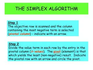
Performing a “Pivot”. Towards a shortcut. z = 2x1 + 3 -z x1 x2 x3 x4 Exercise: to do with your partner. 1 2 0 0 0 -3 = x1 = Dx2 = 1 + 2Dx3 = 7 - 3D. x4 = 5 - 2Dz = 3 + 2D 0 3 0 1 0 7 = = 0 -2 1 0 0 1 0 2 0 0 1 5 = 1. Determine how large D can be.2. Determine the next solution.3. Determine what coefficient should be pivoted on.4. The choice depends on ratios involving the coefficients. What is the rule for determining the coef?
More on performing a pivot • To determine the column to pivot on, select a variable with a positive cost coefficient • To determine a row to pivot on, select a coefficient according to a minimum ratio rule • Carry out a pivot as one does in solving a system of equations.
One more modeling rule: whenever possible, one wants a Linear Program • Suppose x is the total number of chairs produced • Suppose y is the number of black chairs • At least 30% of chairs must be black: y/x 0.30 (assumes x nonzero) This is not linear!!!!! Always transform into a linear constraint: y – 0.30x 0 (works even for x=0!)
Next Lecture • Review of the simplex algorithm • Formalizing the simplex algorithm • How to find an initial basic feasible solution, if one exists • A proof that the simplex algorithm is finite (assuming non-degeneracy)