Download
1 / 29
290 likes | 371 Views
Estimating regional sources and sinks of CO 2 for North America. Using NOAA-CMDL measurements and the TM5 model. Wouter Peters, NOAA CMDL TRANSCOM May 13th, 2003. Acknowledgements. Maarten Krol Pieter Tans Lori Bruhwiler Sander Houweling Peter Bergamaschi Peter van Velthoven

E N D
Estimating regional sources and sinks of CO2 for North America Using NOAA-CMDL measurements and the TM5 model Wouter Peters, NOAA CMDL TRANSCOM May 13th, 2003
Acknowledgements Maarten Krol Pieter Tans Lori Bruhwiler Sander Houweling Peter Bergamaschi Peter van Velthoven Frank Dentener Jan Fokke Meirink John Miller
Outline • My background • The TM5 global & regional model • The expanded NOAA-CMDL network • Plans for inversions • Kalman filter • 4d-var
My background • Master’s in meteorology and physical oceanography from University of Utrecht • Thesis work on LBA-CLAIRE, airborne campaign in Suriname, South America. • PhD on tropospheric ozone in the tropics with Jos Lelieveld and Maarten Krol.
TM3 global model • 5x3.75 degrees, 19 layers • ECMWF meteorology (1979-1993, and 1994-1999) • Full chemistry (O3-NOx-CO-CH4, lumped NMHC’s) + coupled photolysis • Extensive budgets of all processes • Fast parallel version (<2 CPU hrs/yr) allowing multi-year simulations or sensitivity tests
TM5: the next generation • New advection algorithm (Berkvens, Botchev, Krol, Verwer, 2001) allows online nesting of fine-scaled grids within a global domain.
TM5 model – vertical resolution 25 vertical layers ~ 8 layers stratosphere ~ 12 layers free troposphere Hybrid coordinates values for US standard atmosphere ~ 5 layers PBL
TM5 • Contributions from IMAU, KNMI, JRC, and in the near future NOAA. • Most important improvements: meteorological input, coding, chemical boundary conditions. • Special emphasis: ERA40=> re-analysis of ECMWF for 1957-2001. • Resolution up to ECMWF operational
TM5 – latest developments- • Adjoint version of TM5 under con struction • 4d-var scheme from ECMWF implemented and working • Kalman filter (Baker, Bruhwiler, Tans) to be implemented
222Rn simulations at different resolutions Courtesy: H. Sartorius IAR-Freiburg
My plans • Forward modeling of CO2 + isotopes, SF6 • Inverse modeling of CO2 + isotopes • Regional scale sources/sinks over the US • Using vertical profile/ tall tower data • Possibly assist in planning and optimizing network design/sampling strategies
NOAA CMDL goals ??????
Proposed TM5 grid Denver Aspen Grand Junction Pueblo Durango
Fixed-lag Kalman smoother • ‘Batch’ inversion technique using n-months of information at a time (3 < n < 9) • Calculates new fluxes and error estimates for xJ=0 (where x= fluxes and J = cost function) • Balances prior flux estimates against new information from observations using prior flux and model-data mismatch • Computationally efficient for multi-decadal inversions • Details: David Baker’s talk tomorrow
4d-var • Uses steepest descend and the calculated value of xJ to minimize J • value of xJ calculated by adjoint model • Iterative scheme to converge to xJ = 0 • Useful for short time periods and many observations
Gt/yr Gt/yr Seasonal CO2 Flux Estimates Land NCEP (1984-2000) ECMWF (1981-1993) PRIOR Ocean
Annual Average Flux Estimates Land NCEP (1984-2000) ECMWF (1981-1992) PRIOR Ocean
Annual Average Flux Estimates with Cyclic Meteorology Land NCEP (1984-2000) NCEP (1990) PRIOR Ocean
Interface: Mixture between ‘fine’ and ‘coarse’: = + Interface Zoom
XYZV VZYX xyzv vzyx vzyx xyzv Write BC Interface Zoom Update parent