Download
1 / 38
380 likes | 529 Views
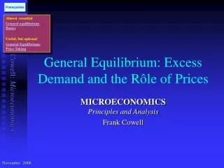
Prerequisites. Almost essential General equilibrium: Basics Useful, but optional General Equilibrium: Price Taking. General Equilibrium: Excess Demand and the R ô le of Prices. MICROECONOMICS Principles and Analysis Frank Cowell. November 2006. Some unsettled questions.

E N D
Prerequisites Almost essential General equilibrium: Basics Useful, but optional General Equilibrium: Price Taking General Equilibrium: Excess Demand and the Rôle of Prices MICROECONOMICS Principles and Analysis Frank Cowell November 2006
Some unsettled questions • Under what circumstances can we be sure that an equilibrium exists? • Will the economy somehow “tend” to this equilibrium? • And will this determine the price system for us? • We will address these using the standard model of a general-equilibrium system • To do this we need just one more new concept.
Overview... General Equilibrium: Excess Demand+ Excess Demand Functions Definition and properties Equilibrium Issues Prices and Decentralisation
Ingredients of the excess demand function • Aggregate demands (the sum of individual households' demands) • Aggregate net-outputs (the sum of individual firms' net outputs). • Resources • Incomes determined by prices check this out
Aggregate consumption, net output • From household’s demand function xih = Dih(p, yh) = Dih(p, yh(p) ) • Because incomes depend on prices • So demands are just functions of p xih = xih(p) • xih(•) depends on holdings of resources and shares • If all goods are private (rival) then aggregate demands can be written:xi(p) = Shxih(p) • “Rival”: extra consumers require additional resources. Same as in “consumer: aggregation” Consumer: Aggregation • From firm’s supply of net output qif = qif(p) • standard supply functions/ demand for inputs Firm and the market graphical summary • aggregation is valid if there are no externalities. Just as in “Firm and the market”) • Aggregate: qi = Sfqif(p)
b a x1 x1 Derivation of xi(p) • Alf’s demand curve for good 1. • Bill’s demand curve for good 1. • Pick any price • Sum of consumers’ demand • Repeat to get the market demand curve p1 p1 p1 x1 Alf Bill The Market
p p p q1 q1+q2 q2 low-cost firm high-cost firm both firms Derivation of qi(p) • Supply curve firm 1 (from MC). • Supply curve firm 2. • Pick any price • Sum of individual firms’ supply • Repeat… • The market supply curve
p1 p1 p1 Resource stock Demand Supply q1 R1 x1 p1 Excess Demand 1 E1 Subtract q and R from x to get E: net output of i aggregated over f demand for i aggregated over h Ei(p) := xi(p) –qi(p) –Ri Resource stock of i
Equilibrium in terms of Excess Demand Equilibrium is characterised by a price vector p* 0 such that: • For every good i: Ei(p*) £ 0 The materials balance condition (dressed up a bit) • For each good i thathas a positive price in equilibrium (i.e. if pi* > 0): Ei(p*) = 0 If this is violated, then somebody, somewhere isn't maximising... You can only have excess supply of a good in equilibrium if the price of that good is 0.
Using E to find the equilibrium • Five steps to the equilibrium allocation • From technology compute firms’ net output functions and profits. • From property rights compute household incomes and thus household demands. • Aggregate the xs and qs and use x, q, R to compute E • Find p* as a solution to the system of E functions • Plug p* into demand functions and net output functions to get the allocation • But this begs some questions about step 4
Issues in equilibrium analysis • Existence • Is there any such p*? • Uniqueness • Is there only one p*? • Stability • Will p “tend to” p*? • For answers we use some fundamental properties of E.
Two fundamental properties... • Walras’ Law. For any price p: n Spi Ei(p) = 0 i=1 You only have to work with n-1 (rather than n) equations Hint #1: think about the "adding-up" property of demand functions... • Homogeneity of degree 0. For any price p and any t > 0: Ei(tp) = Ei(p) You can normalise the prices by any positive number Hint #2: think about the homogeneity property of demand functions... Can you explain why they are true? Link to consumer demand Reminder : these hold for any competitive allocation, not just equilibrium
Price normalisation • We may need to convert from n numbers p1, p2,…pn to n1 relative prices. • The precise method is essentially arbitrary. • The choice of method depends on the purpose of your model. • It can be done in a variety of ways: You could divide by to give a • This method might seem weird • But it has a nice property. • The set of all normalised prices is convex and compact. n Spi i=1 pn a numéraire plabour pMarsBar neat set of n-1 prices standard value system “Marxian” theory of value Mars bar theory of value set of prices that sum to 1
Normalised prices, n=2 • The set of normalised prices p2 • The price vector (0,75, 0.25) • (0,1) J={p: p0, p1+p2= 1} • (0, 0.25) (0.75, 0) p1 • (1,0)
Normalised prices, n=3 p3 • The set of normalised prices • The price vector (0,5, 0.25, 0.25) • (0,0,1) J={p: p0, p1+p2+p3= 1} p2 • (0, 0, 0.25) • (0,1,0) (0, 0.25 , 0) 0 • (1,0,0) (0.5, 0, 0) p1
Overview... General Equilibrium: Excess Demand+ Excess Demand Functions Is there any p*? Equilibrium Issues • Existence • Uniqueness • Stability Prices and Decentralisation
Approach to the existence problem • Imagine a rule that moves prices in the direction of excess demand: • “if Ei >0, increase pi” • “if Ei <0 and pi >0, decrease pi” • An example of this under “stability” below. • This rule uses the E-functions to map the set of prices into itself. • An equilibrium exists if this map has a “fixed point.” • a p* that is mapped into itself? • To find the conditions for this, use normalised prices • p J. • J is a compact, convex set. • We can examine this in the special case n = 2. • In this case normalisation implies that p2 º 1 p1.
Why? Existence of equilibrium? Why boundedness below? As p2 0, by normalisation, p11 As p2 0 if E2 is bounded below then p2E2 0. By Walras’ Law, this implies p1E1 0 as p11 So if E2 is bounded below then E1 can’t be everywhere positive • ED diagram, normalised prices • Excess demand function with well-defined equilibrium price • Case with discontinuous E • Case where excess demand for good2 is unbounded below 1 • E-functions are: • continuous, • bounded below p1 good 2 is free here Excess supply Excess demand • No equilibrium price where E crosses the axis • p1* good 1 is free here E1 0 • E never crosses the axis
Existence: a basic result • An equilibrium price vector must exist if: • excess demand functions are continuous and • bounded from below. • (“continuity” can be weakened to “upper-hemi-continuity”). • Boundedness is no big deal. • Can you have infinite excess supply...? • However continuity might be tricky. • Let's put it on hold. • We examine it under “the rôle of prices”
Overview... General Equilibrium: Excess Demand+ Excess Demand Functions Is there just one p*? Equilibrium Issues • Existence • Uniqueness • Stability Prices and Decentralisation
The uniqueness problem • Multiple equilibria imply multiple allocations, at normalised prices... • ...with reference to a given property distribution. • Will not arise if the E-functions satisfy WARP. • If WARP is not satisfied this can lead to some startling behaviour... let's see
Multiple equilibria • Three equilibrium prices • Suppose there were more of resource 1 • Now take some of resource 1 away 1 p1 'Gone!!' single equilibrium jumps to here!! three equilibria degenerate to one! 'Gone!!' 0 E1
Overview... General Equilibrium: Excess Demand+ Excess Demand Functions Will the system tend to p*? Equilibrium Issues • Existence • Uniqueness • Stability Prices and Decentralisation
Stability analysis • We can model stability similar to physical sciences • We need... • A definition of equilibrium • A process • Initial conditions • Main question is to identify these in economic terms Simple example
A stable equilibrium Equilibrium: Status quo is left undisturbed by gravity Stable: If we apply a small shock the built-in adjustment process (gravity) restores the status quo
An unstable equilibrium Equilibrium: This actually fulfils the definition. But…. Unstable: If we apply a small shock the built-in adjustment process (gravity) moves us away from the status quo
“Gravity” in the CE model • Imagine there is an auctioneer to announce prices, and to adjust if necessary. • If good i is in excess demand, increase its price. • If good i is in excess supply, decrease its price (if it hasn't already reached zero). • Nobody trades till the auctioneer has finished.
“Gravity” in the CE model: the auctioneer using tâtonnement individual dd & ss Announce p individual dd & ss Adjust p individual dd & ss Adjust p individual dd & ss Adjust p …once we’re at equilibrium we trade Evaluate excess dd Equilibrium? Equilibrium? Evaluate excess dd Evaluate excess dd Equilibrium? Evaluate excess dd Equilibrium?
Adjustment and stability • Adjust prices according to sign of Ei: • If Ei > 0 then increase pi • If Ei < 0 and pi > 0 then decrease pi • A linear tâtonnement adjustment mechanism: • Define distance d between p(t) and equilibrium p* • Given WARP, d falls with t under tâtonnement Two examples: with/without WARP
Globally stable... 1 • Start with a very high price • Yields excess supply p1(0) • Under tâtonnement price falls • Start instead with a low price • Yields excess demand Excess demand Excess supply • Under tâtonnement price rises • p1* • p1* • If E satisfies WARP thenthe system must converge... p1 p1(0) E1 0 E1(0) E1(0)
Not globally stable... • Start with a very high price 1 • …now try a (slightly) low price • Start again with very low price p1 Locally Stable • …now try a (slightly) high price • Check the “middle” crossing Excess demand Excess supply • Here WARP does not hold • Two locally stable equilibria • One unstable Unstable Also locally stable 0 E1
Overview... General Equilibrium: Excess Demand+ Excess Demand Functions The separation theorem and the role of large numbers Equilibrium Issues Prices and Decentralisation
Decentralisation • Recall the important result on decentralisation • discussed in the case of Crusoe’s island • The counterpart is true for this multi-person world. • Requires assumptions about convexity of two sets, defined at the aggregate level: • the “attainable set”: A := {x: x £ q+R, F(q) £0 } • the “better-than” set: B(x*) := {Shxh: Uh(xh )³Uh(x*h ) } • To see the power of the result here… • use an “averaging” argument • previously used in lectures on the firm Link to Crusoe: Link to Firm and market
Decentralisation again • The attainable set x2 • The “Better-than-x* ” set • The price line • Decentralisation • A = {x: x q+R, F(q)0} B • B = {Shxh: Uh(xh) Uh(x*h)} • x* • x* maximises income over A p1 p2 • x* minimises expenditure over B A x1 0
Problems with prices • Either non-convex technology (increasing returns or other indivisibilities) for some firms, or... • ...non-convexity of B-set (non-concave- contoured preferences) for some households... • ...may imply discontinuous excess demand function and so... • ...absence of equilibrium. • But if there are are large numbers of agents everything may be OK. two examples
A non-convex technology One unit of input produces exactly one of output • The case with 1 firm B • Rescaled case of 2 firms, output • q' • … 4 , 8 , 16 • Limit of the averaging process • The “Better-than” set • “separating” prices and equilibrium • q* • Limiting attainable set is convex q° • Equilibrium q* is sustained by a mixture of firms at q° and q' . input A
Non-convex preferences • The case with 1 person x2 • Rescaled case of 2 persons, • A continuum of consumers • The attainable set No equilib-rium here • “separating” prices and equilibrium • x' • Limiting better-than set is convex • x* B • Equilibrium x* is sustained by a mixture of consumers at x° and x' . • x° A x1
Summary • Excess demand functions are handy tools for getting results • Continuity and boundedness ensure existence of equilibrium • WARP ensures uniqueness and stability • But requirements of continuity may be demanding Review Review Review Review