Download
1 / 31
310 likes | 482 Views
Neutral Hydrogen at High Redshift. Jared Bowden Dain Kavars. Agenda. Brief introduction and current knowledge N-Body simulations and models Projected integration times Techniques of detection (Instruments) Results and conclusions. Introduction. HI at large z

E N D
Neutral Hydrogen at High Redshift Jared Bowden Dain Kavars
Agenda • Brief introduction and current knowledge • N-Body simulations and models • Projected integration times • Techniques of detection (Instruments) • Results and conclusions
Introduction • HI at large z • HI is uniformly distributed at z >> 20 • Current observations • Show galaxies from z = 5 to 0 • What is going on from z = 20 to z = 5? • HI probes could constrain formation models • When did the IGM become ionized?
Current Knowledge • First star clusters form at z ~ 20 • UV radiation from first generation clusters ionizes HI • IGM is completely ionized at z < 5 • HI exists only in dense clumps due to high column density • No direct observations from z = 20 to z = 5
HI at current epoch • Watch the movie
Phases of HI • Current/Late Epoch (5 < z < 0) • IGM completely ionized • HI exists in dense clumps • Early Epoch (z >> 20) • Uniformly distributed • No ionization
Phases of HI • Intermediate Epoch (20 < z < 5) • Ionized Phase • Same as the current epoch • Warm Phase • HI has been reheated by first stars • No reionization • Spin temperature >> CMB temperature • Observed in redshifted 21 cm radiation
Phases of HI • Intermediate Epoch (20 < z < 5) • Cold Phase • Far from sources of radiation • No reionization, no reheating • Spin temperature ~ CMB temperature • No radiation expected
What We Need to Detect • Need to detect the fluctuations of redshifted 21 cm radiation • Need to predict the detection limit • Use N-Body simulations to generate maps • What instrument could reach that level?
N-Body Simulations • 1283 particles • Each “particle” has M = 2.7 x 10¹¹ Ω0 MSun • 1283 mesh • Physical size = 128 h-1 Mpc • Variety of models can be implemented
Potential Problems • Considering gravity only, no gas pressure • Plays a role in small scale distribution and the state of the gas • But only worried about large scale properties • Assume HI assigned to a particle does not depend on the mass of the collapsed structure that contained it • But we expect large structures to behave like groups of galaxies (i.e. less HI by fraction) • Expect smaller structures to have less HI fraction due to photo-ionizing background
Models • Standard CDM (sCDM) • h = 0.5, Ω0 = 1, Γ= 0.5 • Mixed Dark Matter (MDM) • h = 0.5, Ω0 = 1, Γ= 0.3 • Λ CDM (LCDM) • h = 0.5, ΩΛ = 0.4, Γ= 0.3 • Others • Open CDM, Tilted Einstein DeSitter
z = 0 Solid Line: sCDM Dash: MDM Dot Dash: LCDM z = 3.34
Choosing the Appropriate Model • Reasons LCDM is preferred model • Growth of perturbations slows down at late epochs • Comoving volume enclosed in given solid angle at high redshifts is higher for a universe with nonzero Λ. This yields more emitters, and hence, a higher signal
sCDM MDM LCDM • All for z = 3.34 • MDM has less power at smaller angular scales • sCDM and LCDM have comparable signals • Physical size = 3 h-1 Mpc per pixel • Contour Levels • 15, 30, 60 μJy
Simulated Radio Map for • z = 5.1 • Physical Size = 5 h-1 Mpc per pixel • Contour Levels • 40, 80, 120, 200 μJy
z = 3.34 • z = 5.1 • We see fewer small scale structures in the z = 5.1 • less small scale structures could be detected at larger redshifts, due to instrumental capabilities • using these models, small scale formation may be taking place
Integration Times (GMRT) • Start with the radiometer equation • = (Tsys/T)2/ • For the GMRT: • Converting Signal to Mass
Computing Integration Times • Desire a 3 detection • z = 3 • For GMRT this occurs for 3 – 6’ scales • Requires 100 – 1000 hours for one beam
Are Detections Likely? • Will there be structures in a GMRT beam? • Volume of beam larger than that used in simulations • Volume of beam much larger than volume of fields already observed (LBG’s) • Spikes observed in both of these fields • Conclusion: Spikes will be seen in GMRT beam
Future Telescopes • Current telescopes inadequate • Need something with a larger collecting area and a higher sensitivity • Possibilities: • GMRT – Giant Metre-wave Radio Telescope • SKA – Square Kilometer Array • LOFAR – Low Frequency Array
Instruments - GMRT • Giant Metre-wave Radio Telescope • 30 45m dishes • 50 - 1500 MHz • Located in India, to try to minimize man-made radio interference • At 327 MHz, 8 times more sensitive than VLA • 3 times the collecting area of the VLA
GMRT – Continued • Central array consists 14 dishes in a 1 km2 region • Angular resolution of 60” for lowest frequencies • 435 baselines (VLA has 351)
Instruments - SKA • Square Kilometer Array • Not Completed • .15 – 20 GHz • Array of arrays: approximately 30 200m dishes • Spread over 1000km • Suitable for pencil beam surveys
Instruments - LOFAR • Low Frequency Array • 10 – 240 MHz • 100 antennas in 1 system; 100 systems • Full Operations – 2008 • Spread over 400km • Capable of observing 11 > z > 3.5
Conclusions • Epoch of 20 > z > 5 important in understanding structure formation • No direct observations at z > 5 • At z = 5, IGM is completely ionized • Use N-body simulations to determine predicted flux levels at these epochs • Compare with levels observable using present technology
Conclusions • Present day technology inadequate • Need next generation telescopes • GMRT (fully operational in next few years) • SKA (~15 years) • LOFAR (~2008)