Download
1 / 56
560 likes | 690 Views
Image Matching via Saliency Region Correspondences. Alexander Toshev Jianbo Shi Kostas Daniilidis. IEEE Conference on Computer Vision and Pattern Recognition (CVPR), 2007 . Outline. Introduction Joint-Image Graph (JIG) Matching Model Optimization in the JIG

E N D
Image Matching via Saliency Region Correspondences Alexander Toshev Jianbo Shi Kostas Daniilidis IEEE Conference on Computer Vision and Pattern Recognition (CVPR), 2007
Outline • Introduction • Joint-Image Graph (JIG) Matching Model • Optimization in the JIG • Estimation of Dense Correspondences • Implementation Details • Experiments • Conclusion
Outline • Introduction • Joint-Image Graph (JIG) Matching Model • Optimization in the JIG • Estimation of Dense Correspondences • Implementation Details • Experiments • Conclusion
Introduction • Correspondence estimation is one of the fundamental challenges in computer vision lying in the core of many problems • To find the correspondence of interest points, whose power is in the ability to robustly capture discriminative image structures
Introduction • Feature-based approaches suffer from the ambiguity of local feature descriptors • To address matching ambiguities is to provide grouping constraints via segmentation • Disadvantage:changing drastically even for small deformation of the scene
Introduction Example : Improvement : Matching by modeling in one score function both the coherence of regions
Introduction • A pair of corresponding regions as co-salient define them as follows: • Each region in the pair should exhibit strong internal coherence with respect to the background in the image • The correspondence between the regions from the two images should be supported by high similarity of features extracted from these regions
Outline • Introduction • Joint-Image Graph (JIG) Matching Model • Optimization in the JIG • Estimation of Dense Correspondences • Implementation Details • Experiments • Conclusion
Joint-Image Graph Matching Model • To formalize this model Introduce the joint-image graph (JIG) which contains • vertices the pixels of both images • edges represent intra-image similarities and inter-image feature matches • A good cluster in the JIG consists of a pair of coherent segments describing corresponding scene parts from the two image
Joint-Image Graph Matching Model • In order to combine the robustness of matching via local features with the descriptive power of salient segments • We detect clusters in JIG represents a pair of co-salient regions contains pixels from both images : • coherent and perceptually salient regions in the images (intra-image similarity criterion) • match well according to the feature descriptors (inter-imagesimilarity criterion)
Joint-Image Graph Matching Model • Intra-image similarity :The image segmentation score is the Normalized Cut criterion applied to both segments (2)
Joint-Image Graph Matching Model • Inter-image similarity : • This function measures the strength of the connections between the regions and • Correspondences between pixels are weakly connected with their neighboring pixels – exactly is uncertain • If we use the same indicator vector , then it can be shown that (3)
Joint-Image Graph Matching Model • The correspondence matrix is defined in terms of feature correspondences encoded in a matrix • should select from pixel matches which connect each pixel of one of the images with at most one pixel of the other image • This can be written as
Joint-Image Graph Matching Model • Matching score function we should maximize the sum of the scores in eq. (2) and eq. (3) in the case of pairs of co-salient regions we can introduce indicator vectors packed in matrix we need to maximize subject to
Joint-Image Graph Matching Model • The above optimization problem is NP-hard even for fixed • We relax the indicator vectors to real numbers • Following [12]it can be shown that the problem is equivalent towhereis a matrix containing feature similarities across the images the constraints enforce to select for each pixel in one of the imagesonly one pixel in the another which it can be mapped (4) [12] S. Yu and J. Shi. Multiclass spectral clustering. In ICCV,2003
Outline • Introduction • Joint-Image Graph (JIG) Matching Model • Optimization in the JIG • Implementation Details • Estimation of Dense Correspondences • Experiments • Conclusion
Optimization in the JIG • In order to optimize matching score function we adopt an iterative two-step approach • First step we maximize with respect to for given this step amounts to synchronization of the ’soft’ segmentations of two images based on • Second step, we find an optimal correspondence matrix given the joint segmentation
Optimization in the JIG • Segmentation synchronization • for fixed the optimization problem from eq. (4) can be solved in a closed form – the maximum is attained for eigenvectors of the generalized eigenvalue problem • due to clutter in this may lead to erroneous solutions • assume that the joint ’soft’ segmentation lies in the subspace spanned by the ’soft’ segmentations and of the separate imageswhere are eigenvectors of the corresponding generalized eigenvalue problems for each of the images
Optimization in the JIG • Segmentation synchronization • Hence we can write: ,whereis the joint image segmentation subspace basis and are the coordinates of the joint ’soft’ segmentation in this subspace • With this subspace restriction for V the score function can be written assubject to is the original JIG weight matrix restricted to the segmentation subspaces (5)
Optimization in the JIG • Segmentation synchronization • If we write in terms of the subspace basis coordinates and for both image • then the score function can be decomposed as follows: (6)
Optimization in the JIG • Segmentation synchronizationIn eq. (6) • The first term serves as a regularizer, which emphasizes eigenvectors in the subspaces with larger eigenvaluesdescribing clearer segments • The second term is a correlation between the segmentations of both images weighted by the correspondences inmeasures the quality of the match
Optimization in the JIG • Segmentation synchronization • The optimal in eq. (5) is attained for the eigenvectors of : diagonal matrix with the largest eigenvalues • is a matrix, • In eq. (4) has much higher dimension
Optimization in the JIG • Segmentation synchronization
Optimization in the JIG • Segmentation synchronizationA different view of the above process can be obtained byrepresenting the eigenvectors by their rows: denote by the row of We can assign to each pixel in the image a k-dimensional vector which we will call the embedding vector of this pixel The segmentation synchronization can be viewed as a rotation of the segmentation embeddings of both images such that corresponding pixels are close in the embedding
Optimization in the JIG Figure 4
Optimization in the JIG • Obtaining discrete co-salient regions From the synchronized segmentation eigenvectors we can extract regions : • suppose is the embedding vector of a particular pixel • the binary mask which describes the segment is a column vector defined as • describes a segment in the JIG and represents a pair of corresponding segments in the images • the matching score between segments can be defined as
Optimization in the JIG • Optimizing the correspondence matrixAfter we obtained we seek In order to obtain fast solution we relax the problem by removing the last inequality constrain we denote where is the embedded vector for pixel (eq. (4)) (7)
Optimization in the JIG • Algorithm 1 • Initialize . Compute • Compute segmentation subspaces as the eigenvectors to the largest eigenvalues of • Find optimal segmentation subspace alignment by computing the eigenvectors of • Compute optimal as in eq. (7). • If different from previous iteration go to step 3 • Obtain pairs of corresponding segments is the match score for the co-salient region
Outline • Introduction • Joint-Image Graph (JIG) Matching Model • Optimization in the JIG • Estimation of Dense Correspondences • Implementation Details • Experiments • Conclusion
Estimation of Dense Correspondences • Initially we choose a sparse set of feature matches extracted using a feature detector • In order to obtain denser set of correspondences we use a larger set of matches between features extracted everywhere in the image • Since this set can potentially contain many more wrong matches than , running algorithm 1 directly on does not give always satisfactory results
Estimation of Dense Correspondences • We prune based on the solution by combining • Similarity between co-salient regions obtained for old feature set Using the embedding view of the segmentation synchronization from fig. 4this translates to euclidean distances in the joint segmentation space weighted by the eigenvalues • Feature similarity from new
Estimation of Dense Correspondences • Suppose, two pixels and have embedding coordinates and obtained from • Then following feature similarities embody both requirements from above: • Finally, the entries in are scaled such that the largest value in is 1 • The new co-salient regions are obtained as a solution of
Estimation of Dense Correspondences • Algorithm 2 Matching algorithm • Extract conservatively using a feature detector • Solve using alg. 1 • Extract using features extracted everywhere in the image • Compute and are the rows of Scale such that maximal element in is 1 • Solve using alg. 1
Outline • Introduction • Joint-Image Graph (JIG) Matching Model • Optimization in the JIG • Estimation of Dense Correspondences • Implementation Details • Experiments • Conclusion
Implementation Details • Inter-image similarities • The feature correspondence matrix is based on affine covariant region detector • For comparison, each feature is represented by a descriptor extracted frombe used to evaluate the appearance similarity between two interest points and
Implementation Details • Inter-image similarities • Define a similarity between pixels andlying in the interest point regions: • 1st term measures the appearance similarity between the regions in which and lie • 2nd term measures their geometric compatibility with respect to the affine transformation of to
Implementation Details • Inter-image similarities • Provided, we have extracted two feature sets from and from as described above • the final match score for a pair of pixels equals the largest match score supported by a pair of feature points: • pixels on different sides of corresponding image contours in both images get connected • shape information is encoded in
Implementation Details • Inter-image similarities
Implementation Details • Inter-image similarities • The final is obtained by pruning:retain • For feature extraction we use the MSER detector[12] combined with SIFT descriptor[4] • For the dense correspondences we use features extracted on a dense grid in the image and use the same descriptor [10] T. Tuytelaars and L. V. Gool. Matching widely separated views based on affine invariant regions. IJCV, 59(1):61–85,2004 [4] D. Lowe. Distinctive image features from scale-invariant keypoints. IJCV, 60(2), 91-110, 2004
Implementation Details • Intra-image similaritiesThe matrices for each image are based on intervening contours two pixels and from the same image belong to the same segment if there are no edges with large magnitude, which spatially separate them:
Implementation Details • Algorithm settings • The optimal dimension of the segmentation subspaces in step 2 depends on the area of the segments in the images -- to capture small detailed regions we need more eigenvectors • For the experiments we used • The threshold from is determined so that initially we obtain approx. 200 − 400 matchesfor our experiments it is
Implementation Details • Time complexity • denote bythe time complexity of step 1,2 in alg. 1 corresponds to the complexity of the Ncut segmentation which is [12] • the complexity of line 3 is computing the full SVD of a dense matrix of size • denote the number of interest point matching isline 4 takes • line 6 is
Implementation Details • Time complexity • in alg. 2, we use alg. 1 twice and step 4 is • the total complexity of alg. 1 is • we can precompute the segmentation for an image and use it every time we match this image
Outline • Introduction • Joint-Image Graph (JIG) Matching Model • Optimization in the JIG • Estimation of Dense Correspondences • Implementation Details • Experiments • Conclusion
Experiments • We conduct two experiments: • detection of matching regions • place recognition • datasets :ICCV2005 Computer Vision Contest : Test4 & Final5 • containing each 38 and 29 images of buildings • each building is shown under different viewpoints
Experiments • Detection of Matching Regions
Experiments • Detection of Matching Regions
Experiments • Detection of Matching Regions • detect matching regions, enhance the feature matches, and segment common objects in manually selected image pairs • the 30 matches with highest score in of the output • the top 6 matching regions