Download
1 / 17
170 likes | 350 Views
Emerging Market Finance: Lecture 10: The Real-Option Approach to Valuation in Emerging Markets. The Limitations of Simple NPV. Simple NPV-Analysis: Treat investment as one-off decision: Project stays constant; cannot be adapted. Treat uncertainty as an exogenous factor

E N D
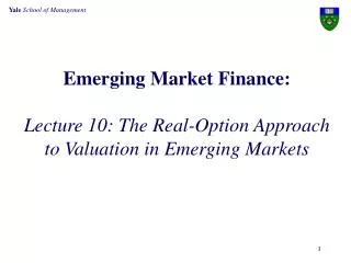
Emerging Market Finance:Lecture 10: The Real-Option Approach to Valuation in Emerging Markets
The Limitations of Simple NPV Simple NPV-Analysis: • Treat investment as one-off decision: • Project stays constant; cannot be adapted. • Treat uncertainty as an exogenous factor Decision Trees and real options • Managers respond to risk-factors: • Integrate strategy and capital budgeting: What is the value of flexibility and responsiveness?
Investment under Uncertainty:The Simple NPV Rule 0 1 2 ... T ... Period Revenue 120 120 ... 120 ... if Demand is high 50% Initial Investment I 50% Revenue if Demand 80 80 ... 80 ... is low Cost of Capital = 10% NPV = - I + 100/0.1 = 1000 - I Invest if I < 1000
Investment under Uncertainty: Delay Strategy: Wait one Period Case 1: I > 800, do not invest if demand is low 0 1 2 ... T ... Period Revenue 0 - I 120 ... 120 ... if Demand is high 50% Demand 50% Revenue if Demand 0 ... 0 ... 0 0 is low 0.5 1200 - I 120 120 (- I + + +... ) = NPV = 1.1 1.12 1.1 2.2
Investment under Uncertainty: Delay (2) Strategy: Wait one Period Case 2: I < 800, always invest 0 1 2 ... T ... Period Revenue 120 ... 120 ... if Demand 0 - I is high 50% Demand 50% Revenue if Demand 80 ... 80 ... 0 - I is low 1 1000 - I 100 100 (- I + + + ... )= NPV = 1.1 1.12 1.1 1.1
Summary of Strategies Decision rule NPV (1) Simple NPV 1000 - I (2) Delay if I > 800 (3) Delay if I < 800 • Delay is never optimal if I < 800 • Delay is better than investing now if I > 833 • Investment is never optimal if I > 1200
Comparison of both Strategies NPV I > 1200: Never invest 833 < I < 1200: Wait; invest if demand is high 1000 I < 833: Invest now 909 1000 - I (1000 - I)/1.1 Vertical distance = value of flexibility 181 (1200-I)/2.2 0 I 0 800 833 1000 1200
Results of Comparison (1) 1 If 833 < I < 1000 Investment now has positive NPV = 1000 - I However: Waiting is optimal in order to see how uncertainty over demand resolves. • Benefits from waiting: receive information to avoid loss. • Costs of waiting: delay of receiving cash flows. Investment in positive NPV projects is not always optimal: the flexibility gained from waiting has a positive value. Note: Critical point is 833, not 800, why?
Results of Comparison (2) 2. If 1000 < I < 1200 Investment now has negative NPV. However: The project should not be abandoned: if demand turns out high later, it has a positive NPV. Negative NPV-projects should be delayed, but not always be dismissed.
Total NPV and Simple NPVIncorporating the Value of Flexibility • The project can be broken down into two components: • The investment possibility itself • Has a Simple NPV of 1000-I • The flexibility of the project from the option to delay investment • Value of Flexibility is: = Max (Value of investment later - Value of investing now, 0) • Total NPV is the value of the whole project: Total NPV = Simple NPV + Value of Flexibility • Investing immediately ignores that option of delay is valuable • Decisions must be based on total NPV The value of flexibility is never negative Total NPV leads always to the correct decision
Compute the Value of Flexibility • If I<833, invest now, hence option to delay has no value. • If 1000>I>833, then: • Value of investing now = 1000 - I • Expected value of investing later is (1200-I)/2.2 • Value of flexibility is then: So, with I=833, the value of flexibility is zero, with I=1000 it increases to 91. • If 1200> I>1000, the value of flexibility is simply (1200-I)/2.2. • How does this change if the investment becomes more risky?
How to Use Total NPV • Assume I=900>833, hence value of flexibility positive. • Value of following optimal strategy = Total NPV • Value of investing now = Simple NPV • Value of flexibility = 80/2.2=36.4 • Should you invest now? • Investing now gives 1000-900=100, • Simple NPV =100>0 • Investing later gives: • Total NPV = Simple NPV + Value of Flexibility = 100 + 36.4 = 136.4 • Total NPV > Simple NPV, therefore delay! • Deciding on the basis of Simple NPV ignores that investing now “kills the option”;
The Impact of Volatility • How does the value of flexibility depend on uncertainty? • Compare previous case with situation of more volatile prices: Revenue (High Demand) = 150 Revenue (Low Demand) = 50 Expected revenue is unchanged ( = 100). • Volatility is higher.
Flexibility in a Volatile Environment Value of Flexibility Prices 150/50 250 Prices 120/80 0 I 0 583 833 1000 1200 1500 Flexibility has a higher value in a more volatile environment
The Option to Abandon Assume same scenario as before, but no option to delay Revenue (High Demand) = 120 Revenue (Low Demand) = 80 Investment outlay I = 1010 If there is no option to delay, NPV=1000-I = -10 • Do not invest! Assume assets have a scrap value: • At the end of the period: scrap value = 910 • After the first period: scrap value = 0
The Option to Abandon High revenue state (120): • PV (Cash Flow) = 1200 > 910 • Continue after period 1! • Receive: 1200 + 120 in period 1 Low revenue state (80): • PV (Cash Flows) = 800 < 910 • Divest and abandon project in period 1! • Receive: 910 + 80 in period 1 With option to abandon, NPV=40 Invest: Option to abandon makes the project viable.
Flexibility and Project Design • Many projects have built-in flexibility: • Options to contract or expand. • Possibility to abandon if the assets have values outside the project (secondary market). • Development opportunities: • Sequence of models of the same product. • Oil fields. • In many cases the project can be designed to be more flexible: • Leasing contracts. • Make or buy decisions. • Scale versus adaptability.