Download
1 / 49
510 likes | 748 Views
Lecture 4 Four transport modelling stages with emphasis on public transport (hands on training). Dr. Muhammad Adnan. Lecture Outline. Trip Generation Trip Distribution Modal Choice Trip Assignment- Car Traffic Trip Assignment – Public transport. Traffic Analysis Zones (TAZs).

E N D
Lecture 4Four transport modelling stages with emphasis on public transport (hands on training) Dr. Muhammad Adnan
Lecture Outline • Trip Generation • Trip Distribution • Modal Choice • Trip Assignment- Car Traffic • Trip Assignment – Public transport
Traffic Analysis Zones (TAZs) • Geographic areas dividing the planning region into relatively similar areas of land use and land activity. Zones represent the origins and destinations of travel activity within the region… every household, place of employment, shopping center, and other activity… are first aggregated into zones and then further simplified into a single node called a centroid. (TRB Report-365) • TAZs serve as the primary unit of analysis in a travel demand forecasting model. They contain socioeconomic data related to land use. TAZs are where trips begin and end
Guidelines for Delineating TAZs • The following can serve as a checklist summarizing recommendations on the best practices in delineating TAZs • The number of people per TAZ should be greater than 1,200, but less than 3,000 for the base and future years; • Each TAZ yields less than 15,000 person trips in the base and future year; • The size of each TAZ is between 0.25 to one square mile in area; • There is a logical number of intrazonal trips in each zone, based on the mix and density of the land use; • Each centroid connector loads less than 10,000 to 15,000 vehicles per day in the base and future year; • The study area is large enough so that nearly all (over 90 percent) of the trips begin and end within the study area; • The TAZ structure is compatible with the base and future year highway and transit network; • The centroid connectors represent realistic access points onto the highway network; • Transit access is represented realistically; • The TAZ structure is compatible with Census, physical, political, and planning district/sector boundaries; • The TAZs are based on homogeneous land uses, when feasible, in both the base and future year • Special generators and freight generators/attractors are isolated within their own TAZ.
Trip Generation • Modelling Methods • Linear regression method • Cross-classification (category analysis) method/trip rate method • _______________________________________________________ • Trip generation • Productions & Attractions • Home-based & non-home based • trips J I Zones
Example • City X has recently conducted a travel survey of its 10 TAZs. The collected data is summarized in the table. Based on the given information • Predict the total number of trips that will be produced by each zone in 10 yrs. (Assume zonal population in 10 yrs is known)? • Relate Y (total trips produced by a zone) to X1 (zonal population)? • Expected total number of trips for a zone with a population of 5,000? • How confident you are about your estimates?
Trip Distribution Models (1) • People decide on Possible destinations is function of • Type and extent of transportation activities • Pattern (location and intensity) of land use • Socio-Economic characteristics of population • Modelling Assumptions • Number of trips decrease with COST between zones • Number of trips increase with zone “attractiveness”
Trip Distribution Models (2) • Growth Factor Models (Uniform, Average Factor, Fratar and Detroit) • Theoretical Models (Gravity Model, Intervening opportunity Model, Entropy Models)
Growth Factor Models (General) • Future trips can be found by proportioning the relative growth in those zones • Iterative in Nature • Start with existing • New proportions established • Iteration continues till we reach stable numbers
Uniform Growth Factor Model F= P*/P0 P* = Design Year Trips P0 = Base year Trips (Total) Tij = F tijfor each pair i and j Tij=Future Trip Matrix tij = Base-year Trip Matrix F= General Growth Rate
Uniform Growth Factor Model The Uniform Growth Factor is typically used for over a 1 or 2 year horizon. However, assuming that trips grow at a standard uniform rate is a fundamentally flawed concept. This method suffers from the disadvantages that it will tend to overestimate the trips between densely developed zones, which probably have little development potential, and underestimate the future trips between underdeveloped zones, which are likely to be extremely developed in the future.
K-Factors • K-factors account for socioeconomic linkages • K-factors are i-j TAZ specific • If i-j pair has too many trips, use K-factor less than 1.0 • Once calibrated, keep constant? for forecast • K-Factors are used to force estimates to agree with observed trip interchanges
Logit Models (Discrete Choice Models) • Binomial Logit Models • Multinomial Logit Models • Nested Logit Models • These models worked on the principle of Random Utility Maximization
Concept of Utility • Utility Function measures the degree of satisfaction that people derive from their choices. • A disutility function represents the generalized cost associated with each choice
Example • Auto Utility Equation: UA= -0.025(IVT) -0.050(OVT) - 0.0024(COST) • Transit Utility Equation: UB= -0.025(IVT) -0.050(OVT) – 0.10(WAIT) – 0.20(XFER) - 0.0024(COST) • Where: • IVT= in-vehicle time in minutes • OVT = out of vehicle time in minutes • COST = out of pocket cost in cents • WAIT = wait time (time spent at bus stop waiting for bus) • XFER = number of transfers • Question: what is the implied cost of IVT? OVT? WAIT? XFER? Binary logit Example
Example • Mode OVT IVT Cost (cents) • 1 person 5 17 200.0 • 2-person carpool 5 21 100.0 • 3-person carpool 5 23 66.6 • 4-person carpool 5 25 50.0 • Transit 7 33 160.0
Part 1: CALCULATE MODE PROBABILITIES BY MARKET SEGMENT • Overview: Calculate the mode probabilities for the trip interchanges. Use the tables on the next pages. • Part A: Calculate the utilities for transit as follows: • Insert in the table the appropriate values for OVT, IVT, and COST. • Calculate the utility relative to each variable by multiplying the variable by the coefficient which is shown in parenthesis at the top of the column; and • Sum the utilities (including the mode-specific constant) and put the total in the last column. • Part B: Calculate the mode probabilities as follows: • Insert the utility for transit in the first column; • Calculate eU for transit • Sum of eU for transit and put in the “Total” column; and • Calculate the probability for transit using the formula: • Sum the probabilities (they should equal 1.0)
Say, from trip distribution, the number of trips was 14,891. Calculate the number of trips by mode using the probabilities calculated. Mode Trips (Zone 5 to Zone 1)
Example-2 • All or Nothing Assignment
Problem formulation • User Equilibrium
For Large Networks- Frank-wolfe Algorithm • Initial UE guess: AON based on free-flow times • Find link travel times at current UE guess • Find Latest AON based on link travel times above • New UE guess: Find best λ to combine old UE guess and latest AON solution through Z function • Repeat second step
O Example -3 D t1(V1)=1+3V1 t2(V2)=2+V2 t3(V3)=3+2V3 O-D Demand constraint V1+V2+V3=10
Solution- FW algorithm • See excel Worksheet • A: Initial estimates of travel time • B: First AON Solution • C: As we don’t yet have any other information, the AON solution in B becomes our first equilibrium flow estimate • D: The corresponding equilibrium travel time estimates are obtained by substituting the flows C in the travel time functions • E: the input travel times to the next step • F: The AON solution • G: This is the first time we have to do some work to calculate these values –the first combination step of the FW algorithm, combination of a mix of C and F • New (V1, V2, V3)= (1-λ)(10,0,0) +λ(0,10,0) = (10-10λ, 10λ, 0), • Put these volumes in Z function, calculate λ, =0.725 GOTO step D and repeat this until travel times equate each other
Transit Assignment • Links include different services running between stops or stations. • Involves movement of passengers, not vehicles • Complex interchange patterns associated with passengers • Impedance functions includes fare structure • Some paths offer more than one parallel service with complex associated choices (e.g., express bus versus local bus service)
Egress time Dwell time Number of transfers Costs • In-vehicle time • Initial wait time • Transfer wait time • Access time To ensure consistency with mode choice, variables used and their weights should be consistent with mode choice utilities
Assignment attributes and weighting factors: • In-vehicle time factor = 1.0 • Auxiliary (walk) travel time factor = 2.0 • Wait time factor = 2.0 • Wait time = Headway/ 2 • Boarding time = 5 min • Boarding time factor =1.0