Download
1 / 34
420 likes | 840 Views
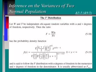
Inference about the ratio of two variances. So far we’ve looked at comparing measures of central location, namely the mean of two populations. When looking at two population variances , we consider the ratio of the variances, i.e. the parameter of interest to us is:

E N D
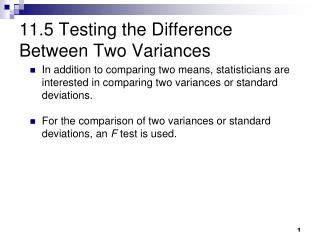
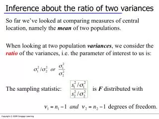
Inference about the ratio of two variances So far we’ve looked at comparing measures of central location, namely the mean of two populations. When looking at two population variances, we consider the ratio of the variances, i.e. the parameter of interest to us is: The sampling statistic: is F distributed with degrees of freedom.
Inference about the ratio of two variances Our null hypothesis is always: H0: (i.e. the variances of the two populations will be equal, hence their ratio will be one) Therefore, our statistic simplifies to:
Example 13.7 IDENTIFY In Example 12.3, we applied the chi-squared test of a variance to determine whether there was sufficient evidence to conclude that the population variance was less than 1.0. Suppose that the statistics practitioner also collected data from another container-filling machine and recorded the fills of a randomly selected sample. Can we infer at the 5% significance level that the second machine is superior in its consistency?
Example 13.7 IDENTIFY The problem objective is to compare two populations where the data are interval. Because we want information about the consistency of the two machines, the parameter we wish to test is σ12 / σ22, where σ12 is the variance of machine 1 and σ22, is the variance for machine 2.
Example 13.7 IDENTIFY We need to conduct the F-test of to determine whether the variance of population 2 is less than that of population 1. Expressed differently, we wish to determine whether there is enough evidence to infer that is σ12 is larger than σ22. Hence the hypotheses we test are H0: σ12 / σ22 = 1 H1: σ12 / σ22 > 1
Example 13.7 COMPUTE For manual calculations
Example 13.7 INTERPRET There is not enough evidence to infer that the variance of machine 2 is less than the variance of machine 1.
Example 13.8 Determine the 95% confidence interval estimate of the ratio of the two population variances in Example 13.7. The confidence interval estimator for σ12 / σ22 is:
Example 13.8 COMPUTE For manual calculations
Example 13.8 COMPUTE Open the F-Estimator_2 Variances worksheet in the Estimators workbook and substitute sample variances, samples sizes, and the confidence level. That is, we estimate that σ12 / σ22 lies between .6164 and 3.1741 Note that one (1.00) is in this interval.
Identifying Factors Factors that identify the F-test and estimator of :
Difference Between Two Population Proportions We will now look at procedures for drawing inferences about the difference between populations whose data are nominal (i.e. categorical). As mentioned previously, with nominal data, calculate proportions of occurrences of each type of outcome. Thus, the parameter to be tested and estimated in this section is the difference between two population proportions: p1–p2.
Statistic and Sampling Distribution… To draw inferences about the the parameter p1–p2, we take samples of population, calculate the sample proportions and look at their difference. is an unbiased estimator for p1–p2. x1 successes in a sample of size n1 from population 1
Sampling Distribution The statistic is approximately normally distributed if the sample sizes are large enough so that: Since its “approximately normal” we can describe the normal distribution in terms of mean and variance… …hence this z-variable will also be approximately standard normally distributed:
Testing and Estimating p1–p2 Because the population proportions (p1 & p2) are unknown, the standard error: is unknown. Thus, we have two different estimators for the standard error of , which depend upon the null hypothesis. We’ll look at these cases on the next slide…
Test Statistic for p1–p2 There are two cases to consider…
Example 13.9 The General Products Company produces and sells a bath soap, which is not selling well. Hoping to improve sales General products decided to introduce more attractive packaging. The company’s advertising agency developed two new designs.
Example 13.9 The first design features several bright colors to distinguish it from other brands. The second design is light green in color with just the company’s logo on it. As a test to determine which design is better the marketing manager selected two supermarkets. In one supermarket the soap was packaged in a box using the first design and in the second supermarket the second design was used.
Example 13.9 The product scanner at each supermarket tracked every buyer of soap over a one week period. The supermarkets recorded the last four digits of the scanner code for each of the five brands of soap the supermarket sold. Xm13-09 The code for the General Products brand of soap is 9077(the other codes are 4255, 3745, 7118, and 8855).
Example 13.9 After the trial period the scanner data were transferred to a computer file. Because the first design is more expensive management has decided to use this design only if there is sufficient evidence to allow them to conclude that it is better. Should management switch to the brightly-colored design or the simple green one?
Example 13.9 IDENTIFY The problem objective is to compare two populations. The first is the population of soap sales in supermarket 1 and the second is the population of soap sales in supermarket 2. The data are nominal because the values are “buy General Products soap” and “buy other companies’ soap.” These two factors tell us that the parameter to be tested is the difference between two population proportions p1-p2 (where p1 and p2 are the proportions of soap sales that are a General Products brand in supermarkets 1 and 2, respectively.
Example 13.9 IDENTIFY Because we want to know whether there is enough evidence to adopt the brightly-colored design, the alternative hypothesis is H1: (p1 – p2) > 0 The null hypothesis must be H0: (p1 – p2) = 0 which tells us that this is an application of Case 1. Thus, the test statistic is
Example 13.9 COMPUTE For manual calculations
Example 13.9 INTERPRET The value of the test statistic is z = 2.90; its p-value is .0019. There is enough evidence to infer that the brightly-colored design is more popular than the simple design. As a result, it is recommended that management switch to the first design.
Example 13.10 Suppose in our test marketing of soap packages scenario that instead of just a difference between the two package versions, the brightly colored design had to outsell the simple design by at least 3%
Example 13.10 IDENTIFY Our research hypothesis now becomes: H1: (p1–p2) > .03 And so our null hypothesis is: H0: (p1–p2) = .03 Since the r.h.s. of H0 is not zero, it’s a “case 2” type problem
Example 13.10 INTERPRET There is not enough evidence to infer that the brightly colored design outsells the other design by 3% or more.
Confidence Interval Estimator The confidence interval estimator for p1–p2 is given by: and as you may suspect, its valid when…
Example 13.11 To help estimate the difference in profitability, the Marketing manager in Examples 13.9 and 13.10 would like to estimate the difference between the two proportions. A confidence level of 95% is suggested.
Example 13.11 COMPUTE For manual calculations
We estimate that the market share for the brightly colored design is between 1.59% and 8.37% larger than the market share for the simple design.
Identifying Factors… Factors that identify the z-test and estimator for p1–p2