Parallel Computers

1. Parallel Computers Chapter 1

2. Parallel Computing • Using more than one computer, or a computer with more than one processor, to solve a problem. Motives • Usually faster computation. • Very simple idea • n computers operating simultaneously can achieve the result faster • it will not be n times faster for various reasons • Other motives include: fault tolerance, larger amount of memory available, ...

3. Parallel programming has been around for more than 50years. Gill writes in 1958*: “... There is therefore nothing new in the idea of parallel programming, but its application to computers. The author cannot believe that there will be any insuperable difficulty in extending it to computers. It is not to be expected that the necessary programming techniques will be worked out overnight. Much experimenting remains to be done. After all, the techniques that are commonly used in programming today were only won at the cost of considerable toil several years ago. In fact the advent of parallel programming may do something to revive the pioneering spirit in programming which seems at the present to be degenerating into a rather dull and routine occupation ...” * Gill, S. (1958), “Parallel Programming,” The Computer Journal, vol. 1, April, pp. 2-10.

4. Some problems needing a large number of computers Computer animation • 1995 - Toy Story processed on 200 processors (cluster of 100 dual processor machines). • 1999 Toy Story 2, -- 1400 processor system • 2001 Monsters, Inc. -- 3500 processors (250 servers each containing 14 processors) Frame rate relatively constant, but increasing computing power provides more realistic animation. Sequencing the human genome • Celera corporation uses 150 four processor servers plus a server with 16 processors. Facts from: http://www.eng.utah.edu/~cs5955/material/mattson12.pdf

5. “Grand Challenge” Problems Ones that cannot be solved in a “reasonable” time with today’s computers. Obviously, an execution time of 10 years is always unreasonable. Examples • Global weather forecasting • Modeling motion of astronomical bodies • Modeling large DNA structures …

6. Weather Forecasting • Atmosphere modeled by dividing it into 3-dimensional cells. • Calculations of each cell repeated many times to model passage of time. Temperature, pressure, humidity, etc.

7. Global Weather Forecasting • Suppose global atmosphere divided into 1 mile  1 mile  1 mile cells to a height of 10 miles - about 5  108 cells. • Suppose calculation in each cell requires 200 floating point operations. In one time step, 1011 floating point operations necessary in total. • To forecast weather over 7 days using 1-minute intervals, a computer operating at 1Gflops (109 floating point operations/s) takes 106 seconds or over 10 days. Obviously that will not work. • To perform calculation in 5 minutes requires computer operating at 3.4 Tflops (3.4  1012 floating point operations/sec) In 2012, a typical Intel processor operates in 20-100 Gflops region, a GPU up to 500Gflops, so we will have to use multiple computers/cores 3.4 Tflops achievable with a parallel cluster

8. “Erik P. DeBenedictis of Sandia National Laboratories theorizes that a zettaFLOPS(ZFLOPS) computer is required to accomplish full weather modeling of two week time span.[1] Such systems might be built around 2030.[2]” Wikipedia “FOPS,” http://en.wikipedia.org/wiki/FLOPS [1] DeBenedictis, Erik P. (2005). "Reversible logic for supercomputing". Proc. 2nd conference on Computing frontiers. New York, NY: ACM Press. pp. 391–402. [2] "IDF: Intel says Moore's Law holds until 2029". Heise Online. April 4, 2008. ZFLOP = 1021 FLOPS

9. Modeling Motion of Astronomical Bodies Each body attracted to each other body by gravitational forces. Movement of each body predicted by calculating total force on each body and applying Newton’s laws (in the simple case) to determine the movement of the bodies.

10. Modeling Motion of Astronomical Bodies • Each body has N-1 forces on it from the N-1 other bodies - O(N) calculation to determine the force on one body (three dimensional). • With N bodies, approx. N2 calculations, i.e. O(N2)* • After determining new positions of bodies, calculations repeated, i.e. N2 x T calculations where T is the number of time steps, i.e. the total complexity is O(N2T). * There is an O(N log2N) algorithm

11. A galaxy might have, say, 1011 stars. • Even if each calculation done in 1 ms (extremely optimistic figure), it takes: • 109 years for one iteration using N2 algorithm or • Almost a year for one iteration using the N log2N algorithm assuming the calculations take the same time (which may not be true). • Then multiply the time by the number of time periods! We may set the N-body problem as one assignment using the basic O(N2) algorithm. However, you do not have 109 years to get the solution and turn it in.

12. Before we embark on using a parallel computer, we need to establish whether we can obtain increased execution speed with an application and what the constraints are. Potential for parallel computers /parallel programming

13. Speedup Factor where ts is execution time on a single processor, and tp is execution time on a multiprocessor. S(p) gives increase in speed by using multiprocessor. Typically use best sequential algorithm for single processor systems. Underlying algorithm for parallel implementation might be (and is usually) different.

14. Parallel time complexity Can extend sequential time complexity notation to parallel computations. Speedup factor can also be cast in terms of computational steps: Although several factors may complicate this matter, including: • Individual processors usually do not operate in synchronism and do not perform their steps in union • Additional message passing overhead

15. Efficiency • If E = 50%  on average, processors are being used half the time • If E = 100%  S(p) = p  all the processors are being used all the times

16. Maximum Speedup Maximum speedup usually p with p processors (linear speedup). Possible to get superlinear speedup (greater than p) but usually a specific reason such as: • System architecture favors parallel formation • Memory for each core is equal  Extra memory in multiprocessor system  less disk memory traffic • Non deterministic algorithm

17. Superlinear Speedup example - Searching (a) Searching each sub-space sequentially Start Time t s t /p s Sub-space D t search x t /p s Solution found x indeterminate

18. (b) Searching each sub-space in parallel D t Speed-up: Solution found

19. Worst case for sequential search when solution found in last sub-space search. Greatest benefit for parallel version Least advantage for parallel version when solution found in first sub-space search of sequential search, i.e. Actual speed-up depends upon which subspace holds solution but could be extremely large non deterministic algorithm

20. Why superlinear speedup should not be possible in other cases: Without such features as a nondeterministic algorithm or additional memory in parallel computer if we were to get superlinear speed up then we could argue that the sequential algorithm used is sub-optimal as the parallel parts in parallel algorithm could simply be done in sequence on a single computer for a faster sequential solution.

21. Maximum speedup with parts not parallelizable (usual case)Amdahl’s law (1967) t s ft (1 - f ) t s s Serial section Parallelizable sections (a) One processor (b) Multiple processors Note the serial section is bunched at the beginning but in practice may be at the beginning, end, and in between p processors (1 - f ) t / p s t p

22. Speedup factor is given by: This equation is known as Amdahl’s law (assuming no overhead) f is the fraction of the computation that cannot be divided into concurrent tasks

23. With an infinite number of processors, maximum speedup is limited to • Example: if only 5% of the computation must be serial / cannot be parallelized  f = 0.05  • Maximum speedup is 20 irrespective of the number of processors • This is a very discouraging result. • Amdahl used this argument to support the design of ultra-high speed single processor systems in the 1960s.

24. Speedup against number of processors f = 0% 20 16 12 f = 5% Speedup factor, S(p) 8 f = 10% f = 20% 4 4 8 12 16 20 Number of processors, p

25. Overhead factors Several factors will appear as overhead in the parallel version and limit the speedup • Periods when not all the processors can be performing useful work (idle) • Extra computations in the parallel version (ex: computing constants locally) • Communication time between processes

26. Gustafson’s law Later, Gustafson (1988) described how the conclusion of Amdahl’s law might be overcome by considering the effect of increasing the problem size. He argued that when a problem is ported onto a multiprocessor system, larger problem sizes can be considered, that is, the same problem but with a larger number of data values.

27. Gustafson’s law Starting point for Gustafson’s law is the computation on the multiprocessor rather than on the single computer. In Gustafson’s analysis, parallel execution time kept constant, which we assume to be some acceptable time for waiting for the solution.

28. Gustafson’s law* Using same approach as for Amdahl’s law: Conclusion- almost linear increase in speedup with increasing number of processors, but fractional sequential part f’needs to diminish with increasing problem size. Example: if f’is 5%, scaled speedup is 19.05 with 20 processors whereas with Amdahl’s law and f = 5% speedup is 10.26. Gustafson quotes results obtained in practice of very high speedup close to linear on a 1024-processor hypercube. * See Wikipedia http://en.wikipedia.org/wiki/Gustafson%27s_law for original derivation of Gustafson's law.

29. Next question to answer is how does one construct a computer system with multiple processors / cores to achieve the speed-up?

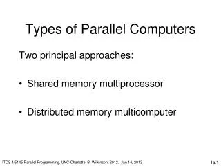
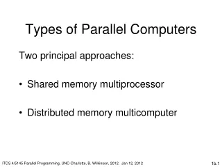
30. Type of Parallel Computers Two principal approaches: • Shared memory multiprocessor • Distributed memory multicomputer

31. Shared Memory Multiprocessor

32. Conventional Computer Consists of a processor executing a program stored in a (main) memory: Each main memory location located by its address. Addresses start at 0 and extend to 2b - 1 when there are b bits (binary digits) in address. Main memory Instr uctions (to processor) Data (to or from processor) Processor

33. Shared Memory Multiprocessor System Natural way to extend single processor model - have multiple processors connected to multiple memory modules, such that each processor can access any memory module: Memory module One address space Processor-memory Interconnections Processors

34. Simplistic view of a small shared memory multiprocessor Examples: • Dual Pentiums • Quad Pentiums Processors Shared memory Bus

35. Real computer system have cache memory between main memory and processors. Level 1 (L1) cache and Level 2 (L2) cache.Example Quad Shared Memory Multiprocessor Processor Processor Processor Processor L1 cache L1 cache L1 cache L1 cache L2 Cache L2 Cache L2 Cache L2 Cache Bus interface Bus interface Bus interface Bus interface Processor/ memory b us Memory controller Memory Shared memory

36. “Recent”innovation • Dual-core and multi-core processors • Two or more independent processors in one package • Actually an old idea but not put into wide practice until recently with the limits of making single processors faster principally caused by: • Power dissipation (power wall) and clock frequency limitations • Limits in parallelism within a single instruction stream • Memory speed limitations (memory wall)

37. Power dissipation Clock frequency “The Free Lunch Is Over: A Fundamental Turn Toward Concurrency in Software” Herb Sutter, http://www.gotw.ca/publications/concurrency-ddj.htm

38. Single “quad core” shared memory multiprocessor Chip Processor Processor Processor Processor L1 cache L1 cache L1 cache L1 cache L2 Cache Memory controller Memory Shared memory

39. Multiple quad-core multiprocessors Processor Processor Processor Processor Processor Processor Processor Processor L2 Cache L1 cache L1 cache L1 cache L1 cache L1 cache L1 cache L1 cache L1 cache possible L3 cache Memory controller Memory Shared memory

40. Programming Shared Memory Multiprocessors Several possible ways – we will concentrate upon using threads Threads - individual parallel sequences (threads), each thread having their own local variables but being able to access shared variables declared outside threads. 1. Low–level thread libraries - programmer calls thread routines to create and control the threads. Example Pthreads, Java threads. 2. Higher level library functions and preprocessor compiler directives - example OpenMP - industry standard. Consists of library functions, compiler directives, and environment variables

41. Tasks – rather than program with threads, which are closely linked to the physical hardware, can program with parallel “tasks”. Promoted by Intel with their TBB (Thread Building Blocks) tools.

42. GPU clusters • Recent trend for clusters – incorporating GPUs for high performance. • GPU often attached through PCI-e x16 interface to CPU, and separate GPU memory. • Now 1000’s cores in each GPU offering orders of magnitude speed improvement for HPC tasks. • 10,000’s of threads possible (Data parallel programming model, see later)

43. Message-Passing Multicomputer

44. Message-Passing Multicomputer Complete computers connected through an interconnection network: Many interconnection networks explored in the 1970s and 1980s including 2- and 3-dimensional meshes, hypercubes, and multistage interconnection networks Interconnection network Messages Processor Local memory Computers

45. Networked Computers as a Computing Platform • Became a very attractive alternative to expensive supercomputers and parallel computer systems for high-performance computing in early 1990s. • Several early projects. Notable: • Berkeley NOW (network of workstations) project. • NASA Beowulf project.

46. Key advantages: • Very high performance workstations and PCs readily available at low cost. • The latest processors can easily be incorporated into the system as they become available. • Existing software can be used or modified.

47. Home-based Beowulf cluster Beowulf Clusters • A group of interconnected “commodity” computers achieving high performance with low cost. • Typically using commodity interconnects - high speed Ethernet, and Linux OS. Beowulf comes from name given by NASA Goddard Space Flight Center cluster project.

48. Cluster Interconnects • Originally fast Ethernet on low cost clusters • Gigabit Ethernet - easy upgrade path More specialized / higher performance interconnects available including Myrinet and Infiniband.

49. Dedicated cluster with a master node and computer nodes User Computers Dedicated Cluster External network Ethernet interface Master node Switch Local network Compute nodes

50. Software Tools for Clusters • Based upon message passing programming model • User-level libraries provided for explicitly specifying messages to be sent between executing processes on each computer . • Use with regular programming languages, for example: • C, C++ • Fortran • MatLab • Java • .NET (Async & Task Parallel Library) • Intel Parallel Studio (Intel threading building blocks) • dRuby (distributed Ruby extension) • Ada • OpenCL (Open Computing Language) • Haskell • Python • LISP