Download
1 / 16
160 likes | 204 Views
Learn about minimizing least squares error in discrete data approximation using polynomials. Study linear independence in orthogonal polynomials.

E N D
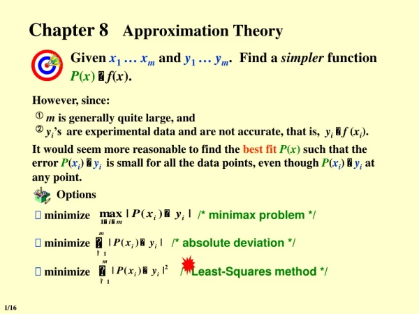
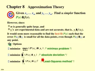
Given x1 … xmand y1 … ym. Find a simpler function P(x) f(x). Options minimize /* minimax problem */ minimize /* absolute deviation */ minimize /* Least-Squares method */ Chapter 8Approximation Theory However, since: ①m is generally quite large, and ②yi’s are experimental data and are not accurate, that is, yi f (xi). It would seem more reasonable to find the best fitP(x) such that the error P(xi) yi is small for all the data points, even though P(xi) yi at any point. 1/16
Chapter 8 Approximation Theory -- Discrete Least Squares Approximation Determine the polynomial Pn(x) = a0 + a1x + … + anxn to approximate a set of data { (xi , yi) | i = 1, 2, …, m } such that the least squares error is minimized. Here n<<m. E2 is actually a function of a0, a1, …, an. That is, [ ]. m 2 = + + + - n ( a , a , ... , a ) a a x ... a x y E2 0 1 0 1 n i n i i = 1 i For E2 to be minimized it is necessary that m n = - j k 2 [ a x y ] x j i i i = = 1 0 i j n m m + = - j k k 2 a x y x j i i i = = = 0 1 1 j i i m m Let = = k k b x , c y x k i k i i = = 1 i 1 i 8.1 Discrete Least Squares Approximation a0a1an Normal equations. A unique solution exists if xiare distinct. 2/16
Chapter 8 Approximation Theory -- Discrete Least Squares Approximation Note: The order of Pn(x) is given by user and must be no larger than m1. If n=m1, then Pn(x) is the Lagrange interpolating polynomial with E2 = 0. P(x) is not necessarily a polynomial. HW: p.494 #5 3/16
Chapter 8 Approximation Theory -- Discrete Least Squares Approximation y x x = y P ( x ) Method 1:Let + ax b m xi = - 2 ( yi ) E2 ( a , b ) axi+b = 1 i Linearization: Let , then Y a + bX is a linear problem. Find a and b such that is minimized. Example: (xi , yi) , i = 1, 2, …, m Take it easy! We just have to linearize it … But hey, the system of equations for a and b is nonlinear! Convert ( xi , yi ) into ( Xi , Yi ), a and b can be solved. 4/16
Chapter 8 Approximation Theory -- Discrete Least Squares Approximation b - ln y ln a x 1 = = = = - Y ln y , X , A ln a , B b x = - / b x y P ( x ) a e Method 2:Let is a linear problem + Y A BX Linearization: Convert ( xi , yi ) into ( Xi , Yi ), a and b can be solved. 5/16
Chapter 8 Approximation Theory -- Orthogonal Polynomials and Least Squares Approximation Given x1 … xmand y1 … ym. Find a simpler function P(x) f(x) such that is minimized. Given a function f(x) defined on [a, b]. Find a simpler function P(x) f(x) such that is minimized. 8.2 Orthogonal Polynomials and Least Squares Approximation Definition: The set of functions { 0(x), 1(x), … , n(x) } is said to be linearly independent on [a, b] if, whenever a00(x)+a11(x)+… +ann(x)=0 for all x[a, b], we have a0= a1=… =an=0. Otherwise the set of functions is said to be linearly dependent. 6/16
Chapter 8 Approximation Theory -- Orthogonal Polynomials and Least Squares Approximation P(x) is a zero polynomial. The coefficient of xn is zero. an= 0 an–1= 0 a0= 0 P(x) = a00(x)+ … +an–1n –1(x) = 0 Theorem: If j(x) is a polynomial of degree j for each j = 0, …, n, then { 0(x), 1(x), … , n(x) } is linearly independent on any interval [a, b]. Proof:If not, then there exist a0, a1, … an such that P(x) = a00(x)+a11(x)+… +ann(x)=0 for all x[a, b]. … … 7/16
Chapter 8 Approximation Theory -- Orthogonal Polynomials and Least Squares Approximation Definition: For a general linear independent set of functions { 0(x), 1(x), … , n(x) }, a linear combination of0(x), 1(x), … , n(x), is called a generalized polynomial. Other polynomials Theorem: Let n be the set of all polynomials of degree at most n. If { 0(x), 1(x), … , n(x) } is a collection of linearly independent polynomials in n, then any polynomials in n can be written uniquely as a linear combination of0(x), 1(x), … , n(x). { j(x) = cos jx }、{ j(x) = sin jx } { j(x), j(x)} generatestrigonometric polynomial. { j(x) = e kj x , ki kj} generatesexponential polynomial. 8/16
Chapter 8 Approximation Theory -- Orthogonal Polynomials and Least Squares Approximation An integrable function w is called a weight function on the interval I if w(x) 0 for all x in I, but w(x) does not vanish on any subinterval of I. We are to consider minimizing . Definition: The weight function ①discrete type When approximating a set of discrete points (xi , yi) for i = 1, …, n, we assign each error term a positive real number wi. That is, to consider minimizing E = wi [ P(xi) – yi]2. The set of {wi} is called the weight. The purpose of the weight is to assign varying degrees of importance to approximations on certain points. ②continuous type 9/16
Chapter 8 Approximation Theory -- Orthogonal Polynomials and Least Squares Approximation Given a function f(x) and a weight function w(x) defined on an interval [a, b]. Find a generalized polynomial P(x) such that the error is minimized. b = - 2 E w ( x )[ P ( x ) f ( x )] dx a Definition: The general least squares approximation problem: ①discrete type Given a set of discrete points (xi , yi) and a set of weights {wi} for i = 1, …, m. Find a generalized polynomial P(x) such that the error E = wi [ P(xi) – yi]2 is minimized. ②continuous type 10/16
Chapter 8 Approximation Theory -- Orthogonal Polynomials and Least Squares Approximation Let P(x) =a00(x)+a11(x)+… +ann(x). Then similar to the discrete problem: n j j = j = ( , ) a ( , f ) , k 0 , ... , n k j j k = 0 j j a ( , f ) 0 0 = c = = j j b ( , ) That is, ij i j j a ( , f ) n n Inner product and Norm It can be shown that ( f, g ) is an inner product and is a norm. f and g are said to be orthogonal if ( f, g )=0. The general least squares approximation problem is to find a generalized polynomial P(x) such that E = (P – y, P – y) = || P – y ||2 is minimized. normal equations 11/16
Chapter 8 Approximation Theory -- Orthogonal Polynomials and Least Squares Approximation Example: Approximate with and w 1. 63 - = 1 || B || || B || = 484, K ( B ) = 7623 4 It is soooo simple! What can possibly go wrong? Solution:0(x) = 1, 1(x) = x, 2(x) = x2 12/16
Chapter 8 Approximation Theory -- Orthogonal Polynomials and Least Squares Approximation Then Improvement: Theorem: The set of polynomial functions { 0(x), 1(x), … , n(x)} defined in the following way is orthogonal on [a, b] with respect to the weight function w. where Example: When approximating f(x) C[0, 1] with j(x) = x j and w(x) 1… Hilbert Matrix! If we can find a general linear independent set of functions { 0(x), 1(x), … , n(x)} such that any pair of i(x) and j(x) are orthogonal, then the normal matrix will be diagonal! In this case we have ak = Well, no free lunch anyway… Construction of the orthogonal polynomials 13/16
Chapter 8 Approximation Theory -- Orthogonal Polynomials and Least Squares Approximation Example: Approximate with and w 1. j = ( x ) 1 0 j ( , y ) 29 = = 0 a 5 j = - B = - 0 j j ( x ) ( x ) x ( , ) 2 j j j j j ( ( x x , , ) ) ( , y ) 37 5 5 1 1 0 0 = = B B = = = = 2 1 a 1 0 0 1 1 j j 2 1 j j j j ( , ) 5 ( ( , , ) ) 2 2 xj1 j ( , ) 5 1 1 1 0 0 1 C = = 0 2 j j ( , ) 4 0 0 j 5 5 ( , y ) 1 = = j = - j - j = - + 2 2 a ( x ) ( x ) ( x ) ( x ) x 5 x 5 2 2 1 0 j j ( , ) 2 2 4 2 2 Solution:Firstconstruct the orthogonal polynomials 0(x), 1(x), 2(x). Let y =a00(x)+a11(x)+ a22(x) 14/16
Chapter 8 Approximation Theory -- Orthogonal Polynomials and Least Squares Approximation Algorithm: Orthogonal Polynomials Approximation To approximate a given function by a polynomial with error bounded by a given tolerance. Input: number of data m; x[m]; y[m]; weight w[m]; tolerance TOL; maximum degree of polynomial Max_n. Output: coefficients of the approximating polynomial. Step 1 Set 0(x) 1; a0 = (0, y)/(0, 0); P(x) = a0 0(x); err = (y, y) a0 (0, y); Step 2 Set B1=(x0, 0)/(0, 0); 1(x)= x B1; a1 = (1, y)/(1, 1); P(x) += a1 1(x); err= a1 (1, y); Step 3 Set k = 1; Step 4 While (( k < Max_n)&&(|err|TOL)) do steps 5-7 Step 5 k ++; Step 6 Bk=(x1, 1)/(1, 1); Ck= (x1, 0)/(0, 0); 2(x)= (x Bk) 1(x) Ck0(x); ak= (2, y)/(2, 2); P(x) += ak2(x); err= ak(2, y); Step 7 Set 0(x) = 1(x); 1(x) = 2(x); Step 8 Output ( ); STOP. 15/16
Chapter 8 Approximation Theory -- Orthogonal Polynomials and Least Squares Approximation Another von Neumann quote : Young man, in mathematics you don't understand things, you just get used to them. Lab 07. Orthogonal Polynomials Approximation Time Limit: 1 second; Points: 4 Given a function f and a set of 200 m > 0 distinct points x1 < x2 < … xm. You are supposed to write a function void OPA ( double (*f)(double x), double x[], double w[], int m, double tol ) to approximate the function fby an orthogonal polynomial using the exact function values at the given m points x[ ]. The array w[m] contains the values of a weight function at the given points x[ ]. The total error must be no larger than tol. HW: p.506 #3, 11 16/16