Download

1 / 17
170 likes | 230 Views
Learn how to calculate the shape of a polynomial based on regression coefficients, specifying polynomial models, solving for values of the independent variable, predicting values, and visualizing the polynomial using a spreadsheet or chart.

E N D
Calculating the shape of a polynomial from regression coefficients Jane E. Miller, PhD
Overview • Functional form of a polynomial • Solving a polynomial for values of the independent variable • Illustrative example • Calculations • Chart • Spreadsheet to perform calculations
Specifying a model with a polynomial • To specify a polynomial function of an independent variable (IV), include linear and higher-order terms for that IV in the model. E.g., • A quadratic specification will include linear and square terms (variables): Y = β0 + β1X1+ β2X12 • A cubic specification will include linear, square, and cubic terms: y = β0 + β1X1+ β2X12+ β3X13
Example: Birth weight as a quadratic function of IPR • If a birth weight model includes both income-to-poverty ratio (IPR) and IPR2 as independent variables, it yields the following quadratic specification: Birth weight = β0 + (βIPR × IPR) + (βIPR2 × IPR2) • βIPR is the coefficient on the linear term • βIPR2 is the coefficient on the square term • IPR is the value of the income-to-poverty ratio variable for each case • IPR2 is IPR-squared for each case
Solving a polynomial based on βs • Birth weight (grams) = β0+ (βIPR× IPR) + (βIPR2 × IPR2) • Substituting the estimated βs into the general equation gives: Birth weight (grams) = 3,317.8 + (80.5IPR) + (–9.9 IPR2) • Which can be solved for specific values of IPR • Estimated coefficients are shown in table 9.1 of The Chicago Guide to Writing about Multivariate Analysis, 2nd Edition.
Calculating the shape of the polynomial, holding constant all other IVs • To calculate the effect of the IV in the polynomial holding constant all other independent variables in the model • The intercept (β0) and the βis related to other IVs in the model will cancel out when you subtract to calculate the difference between values. • So you don’t have to include those coefficients in these calculations.
Calculating predicted values of the dependent variable (DV) for different values of the IV • Solve the equation (80.5IPR) + (–9.9 IPR2) for each of several selected values of X1. E.g., • At IPR = 1.0 • Birth weight = (80.5 1.0) + (–9.9 1.02) = 70.6 grams • At IPR = 2.0 • Birth weight = (80.5 2.0) + (–9.9 2.02) = 121.4 grams • At IPR = 3.0 • Birth weight = (80.5 3.0) + (–9.9 3.02) = 151.8 grams βIPR = 80.5; βIPR2 = –9.9. We ignore β0because it cancels out when we subtract to calculate differences across predicted values, in the next step.
Selecting values of the IV for which to calculate the predicted DV • Select values of the IV to solve for by picking 5 or 6 values that span the observed range of Xi in your data. E.g., • The income-to-poverty ratio (IPR) ranges from 0 to 5, so plug in values at 1-unit increments across that range. • Mother’s age ranges from 15 to 49, so if your model specifies a polynomial function of age, solve it for values at 5-year increments across that range. • Avoidselectingout of range values, since they were not included in the model that estimated the βs.
Calculating the effect of changes in the IV on the DV • Compute the difference in predicted value of the dependent variable (DV, Y) by subtracting predicted values of Y for different values of the IV (Xi). • E.g., predicted Y (Xi = 2) – predicted Y (Xi = 1) • Important to do this for several pairs of values of the IV because when the association is specified with a polynomial, by definition, Xi will not have a constant marginal effect on Y.
Example: Birth weight as a quadratic function of IPR • As we saw earlier: • At IPR = 1.0, predicted birth weight = 70.6 grams • At IPR = 2.0, predicted birth weight = 121.4 grams • At IPR = 3.0, predicted birth weight = 151.8 grams • Thus the marginal effect of moving from IPR = 1.0 to IPR = 2.0 is 121.4 – 70.6 = 50.8 grams IPR = 2.0 to IPR = 3.0 is 151.8 – 131.4 = 30.4 grams
Coefficients and shape of the quadratic • In this example, the decreasing marginal positive effect of IPR on birth weight is due to the combination of • a positive βIPR • a negativeβIPR2 • Recall: βIPR = 80.5; βIPR2 = –9.9 • Other combinations of positive and negative signs on the linear and squared terms will generate different shapes of the quadratic function.
Using a spreadsheet to calculate pattern of a polynomial from βs • Spreadsheets are well-suited to conducting repetitive, multistep calculations. • Type in: • Estimated coefficients on the polynomial terms, • Selected values of the independent variable, • Formulas to calculate predicted value of the dependent variable from the βs and values of the independent variable (IV). • Generalize the formulas to apply to all values of the IV. • Create a chart to portray the association between the IV and DV across the observed range of the IV.
Summary • A regression model involving a polynomial will include separate variables for each term in the polynomial. • The overall shape of the pattern can be calculated by solving the polynomial for values of: • The estimated coefficients on the polynomial terms, and • Selected values of the independent variable across its observed range in the data. • A spreadsheet is an efficient way to calculate and graph the polynomial.
Suggested resources • Miller, J. E. 2013. The Chicago Guide to Writing about Multivariate Analysis, 2nd Edition. • Chapter 10, section on polynomials • Appendix D, using a spreadsheet for calculations • Podcast on • Interpreting regression coefficients • Spreadsheet templates • Spreadsheet basics • Solving for a quadratic
Suggested practice exercises • Study guide to The Chicago Guide to Writing about Multivariate Analysis, 2nd Edition. • Suggested course extensions for chapter 10 • “Applying statistics and writing” question #7. • “Revising” questions #6 and 9.
Contact information Jane E. Miller, PhD jmiller@ifh.rutgers.edu Online materials available at http://press.uchicago.edu/books/miller/multivariate/index.html