Download
1 / 45
450 likes | 503 Views
Explore the properties and applications of Butterworth, Chebyshev, Elliptic, and Bessel filters in signal processing. Learn about their characteristics, designs, and frequency response for noise removal and signal enhancement. Dive into analog lowpass filter design techniques and practical implementations.

E N D
3.4 Frequency-domain Filters Commonly used filters * Butterworth filters * Elliptic filters * Chebyshev filters * Bessel filters a type of linear filter with a maximally flat group delay (maximally linear phase response). Bessel filters are often used in audio crossover systems.
Maturity in analog lowpass filter design (1. (2. (3.
3.4.1 Removal of high-frequency noise: Butterworth lowpass filters Properties of Butterworth filters: 1. Most commonly used frequency-domain filters 2. Simplicity 3. A maximally flat magnitude response in the pass-band 4. 2N 1 derivatives of the squared magnitude response at ( = 0) = 0, for Butterworth lowpass filter of order N 5. Monotonic filter response in the pass-band and the stop-band 6. The squared transfer function |Ha(j)|2 =1/[1+( j/jc)2N] Ha: the frequency response of the analog filter c: the cutoff frequency (in radians/s) 7. Completely specified by the cutoff frequency c and the order N. 8. N increases more flat pass-band response; sharper pass-band to stop-band transition
Properties of Butterworth filters: 9. |Ha(jc)|2 = 1/2 for all N 10. The squared transfer function Ha(s) Ha(s) =1/[1+( s/jc)2N] 11. The poles of the squared transfer function sk = c exp{j[1/2 + (2k 1) / 2N]}, k = 1, 2, 3, …, 2N (a) For the filter coefficients to be real complex poles must appear in conjugate pairs (b) For a stable and causal responser Ha(s) only has poles on the left-hand side of the s-plane Ha(s) = G/[(sp1) (sp2) (sp3)…(spN)] 12. By using the bilinear transform s = (2/T)[(1 z1)/(1 + z1)] to map Ha(s) to the z-domain, H(z) = G’(1 + z 1)N/(Nk = 0 ak zk), k = 0, 1, 2, …, N a0 = 1 G’ is such that H(z) = 1 at z = 1, i.e., at DC y(n) = Nk = 0 bk x(n-k) - Nk = 0 ak y(n-k) 13. H(z) is an IIR filter
Step 1 1.
Step 2: Pole locations S(1) = -0.5561 + 1.3425i S(2) = -1.3425 + 0.5561i S(3) = -1.3425 - 0.5561i S(4) = -0.5561 - 1.3425i S(5) = 0.5561 - 1.3425i S(6) = 1.3425 - 0.5561i S(7) = 1.3425 + 0.5561i S(8) = 0.5561 + 1.3425i
Step 3: Form Ha(s) Choose s(1:4) as the poles for Ha(s) Ha(s) = 分子 /(s – s(1)) (s – s(2)) (s – s(3)) (s – s(4)) Ha(s) = 1 @ DC , so the 分子 = 2.111456 * 2.111456 = 4.458247 Ha(s) = 4.458247 /(s – s(1)) (s – s(2)) (s – s(3)) (s – s(4)) (equation 3.62)
S = (2/T)(1-z-1)/(1+z-1) • Ha(s) = 4.458247 /(s – s(1)) (s – s(2)) (s – s(3)) (s – s(4)) • H(z) = Equation 3.63 • b = [0.0465829, …. • a = [1, -0.776740, ….. • Use [h,w] = freqz(b,a) • fs = 200; • a = [1, -0.776740, 0.672706, -0.180517,0.029763]; • b = [0.0465829, 0.186332,0.279497,0.186332,0.046583]; • % a = [1.0000 -0.7767 0.6727 -0.1805 0.0298]; • % b= [0.0466 0.1863 0.2795 0.1863 0.0466]; • [h,w] = freqz(b,a); • subplot(2,1,1); • plot(w*(fs/2)/pi,abs(h));xlabel('Frequency, Hz'); ylabel('Magnitude'); grid; • subplot(2,1,2); • plot(w*(fs/2)/pi,angle(h) * 180 / pi); xlabel('Frequency, Hz'); ylabel('Phase, degree'); grid; • fvtool(b,a); Sep 4: Bilinear transform
[b,a] = butter(4,0.4); fvtool(b,a); % The four zeros are at the same location.
a = [1, -0.776740, 0.672706, -0.180517,0.029763]; b = [0.0465829, 0.186332,0.279497,0.186332,0.046583]; fvtool(b,a);
a = [1.0000 -0.7767 0.6727 -0.1805 0.0298]; b= [0.0466 0.1863 0.2795 0.1863 0.0466]; fvtool(b,a);
Step 5 y(n) = Nk = 0 bk x(n-k) - Nk = 0 ak y(n-k) (Equation 3.59)
Homeworkdue on 2009.11.16 (Monday midnight) Design a Butterworth LPF with N = 4, fc = 50 Hz. (fs = 200 Hz) (i) Ha(s) = ? (ii) H(z) = ? (iii) Plot the magnitude response and the phase response. Put the answers in a Word file and turn in on the Black Board System before the midnight of 2009.11.16.
Design by Matlab B = [0.0466 0.1863 0.2795 0.1863 0.0466] A = [1.0000 -0.7821 0.6800 -0.1827 0.0301] H(z) = (0.0466 + 0.1863 z-1 + 0.2795 z-2 + 0.1863 z-3 + 0.0466 z-4) / (1.0000 - 0.7821 z-1 + 0.6800 z-2 - 0.1827 z-3 0.0301 z-4)
To compensate for the distortion caused by bilinear transform
Figure 3.06(Original ECG signal with baseline wandering Figure 3.27(Output of derivative-based time-domian highpass filter as shown in Figure 3.27 Figure 3.38(Output of Butterworth highpass filter
Figure 3.27 Figure 3.39