Download
1 / 15
290 likes | 692 Views
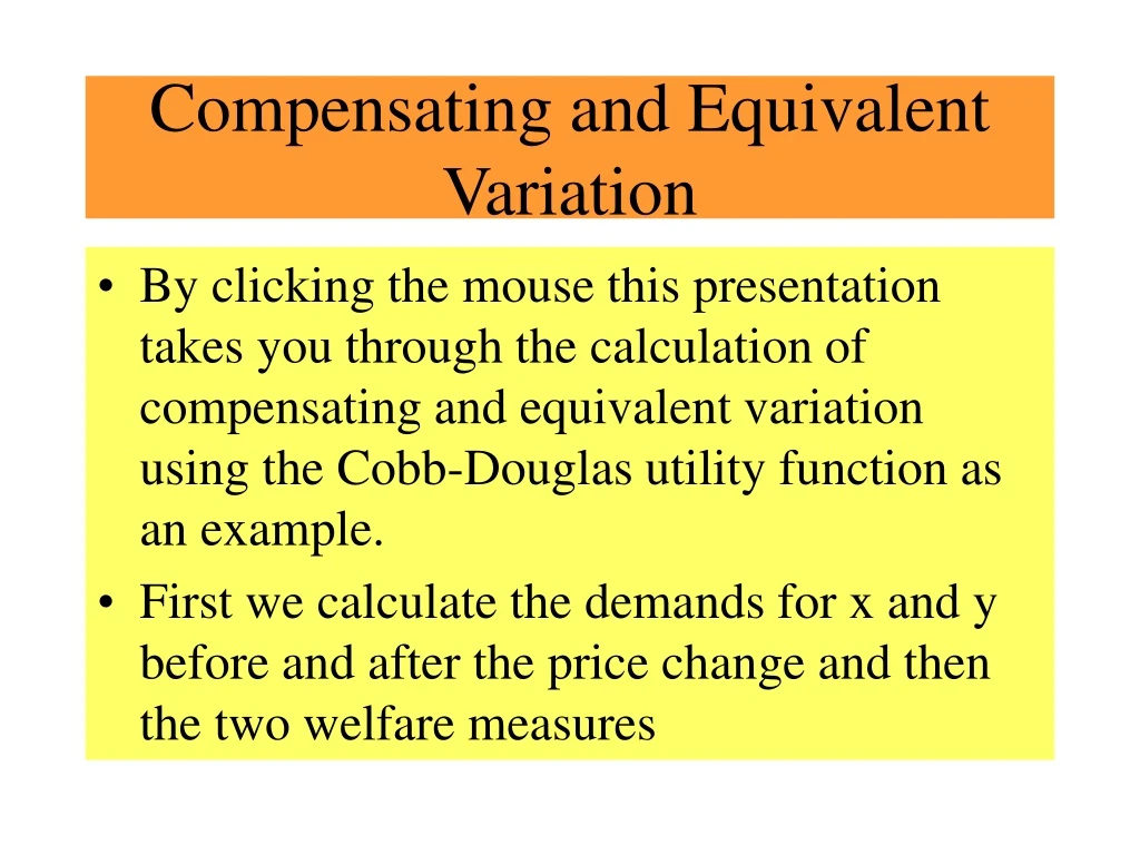
Compensating and Equivalent Variation. By clicking the mouse this presentation takes you through the calculation of compensating and equivalent variation using the Cobb-Douglas utility function as an example.

E N D
Compensating and Equivalent Variation • By clicking the mouse this presentation takes you through the calculation of compensating and equivalent variation using the Cobb-Douglas utility function as an example. • First we calculate the demands for x and y before and after the price change and then the two welfare measures
The demand functions when utility is Cobb-Douglas We know that for Cobb-Douglas Utility functions with U = xayb that the demand function are:
Suppose we assume that M = 100, p1=1 & p2=1 then with U(x,y) = x1/2 y1/2, that is a=b=1/2
So the initial demands for x and y with the price of x =1 ,price of y=1 and M= 100are: • xd = 50 and yD = 50
Suppose we increase the price of x, what will the demand for x and y be now?
Using our Cobb-Douglas demand functions we can calculate the new demand for x (and y) If pxrises to2 then x = 25 and y = 50
Compensating Variation • To calculate this we need to calculate the income required to ensure that we can reach the original utility at the new set of prices. • The original utility was U(50,50)=501/2 501/2 • U(50,50)=(50.50)1/2 (50 2 )1/2 = 50
y 50 25 50 Next we need to find the income that must be given back to a consumer to compensate him or her for the rise in prices.
What level of Income gives Utility =50 at the new prices? • To find this out we can use the demand functions we have derived for x and y. • Next we substitute these demands (using the new prices (2,1) directly into the utility function and set it equal to U0
Equivalent Variation WE find this in a similar manner to compensating variation except that now we want to find the income required to ensure that we are at the new level of utility but with the old set of prices. The new level of utility is: U(25,50) = 251/2501/2
y Thus diagram shows the amount of income we need to take away from the consumer at the old set of prices to bring them to the new utility level. 50 U1=50 Uo=35.5 25 50
Equivalent Variation Once again we find the Income which will give us this Utility at the old prices.
Result • Compensating Variation = 141 • Equivalent Variation =70.7 • and since price has risen CV>EV as we saw in lectures