Download
1 / 51
1.03k likes | 2.61k Views
IMPEDANCE TRANSFORMERS AND TAPERS. Lecturers: Lluís Pradell ( pradell@tsc.upc.edu ) Francesc Torres (xtorres@tsc.upc.edu). March 2010. The quarter-Wave Transformer* ( i ). A quarter-wave transformer can be used to match a real impedance Z L to Z 0. Z in. Z 0. Z 1. Z L.

E N D
IMPEDANCE TRANSFORMERS AND TAPERS Lecturers: Lluís Pradell (pradell@tsc.upc.edu) Francesc Torres (xtorres@tsc.upc.edu) March 2010
The quarter-Wave Transformer* (i) A quarter-wave transformer can be used to match a real impedance ZL to Z0 Zin Z0 Z1 ZL If The matching condition at fo is At a different frequency and the input reflection coefficient is The mismatch can be computed from: *Pozar 5.5
The quarter-Wave Transformer (ii) If Return Loss is constrained to yield a maximum value , the frequency that reaches the bound can be computed from: Where for a TEM transmission line And the bound frequency is related to the design frequency as:
The quarter-Wave Transformer (iii) Finally, the fractional bandwdith is given by
Multisection transformer* (i) The theory of small reflections In the case of small reflections, the reflection coefficient can be approximated taking into account the partial (transient) reflection coefficients: That is, in the case of small reflections the permanent reflection is dominated by the two first transient terms: transmission line discontinuity and load *Pozar 5.6
Multisection transformer (ii) The theory of small reflections can be extended to a multisection transformer It is assumed that the impedances ZN increase or decrease monotically The reflection coefficients can be grouped in pairs (ZN may not be symmetric)
Multisection transformer (iii) The reflection coefficient can be represented as a Fourier series for N even for N odd Finite Fourier Series: periodic function (period: q = p) • Any desired reflection coefficient behaviour over frequency can be synthesized by properly choosing the coefficients and using enough sections: • Binomial (maximally flat) response • Chebychev (equal ripple) response
Binomial multisection matching transformer (i) Binomial function The constant A is computed from the transformer response at f=0: The transformer coefficients are computed from the response expansion: The transformer impedances Zn are then computed, starting from n=0, as:
Binomial multisection matching transformer (iii) 1 Bandwidth of the binomial transformer The maximum reflection at the band edge is given by: The fractional bandwitdh is then:
Chebyshev multisection matching transformer Chebyshev polynomial
Chebyshev transformer design Application: Microstrip to rectangular wave-guide transition: both source and load impedances are real. Ridge guide section Microstrip line Steped ridge guide Rectangular guide Ridge guide: five λ/4 sections: Chebychev design
TRANSFORMER EXAMPLE (1):ADS SIMULATION Chebyshev transformer, N = 3, |GM|=0.05 (ltotal = 3l/4) 57,37 W 70,71 W 87,14 W 100 W 50 W
TRANSFORMER EXAMPLE (2):ADS SIMULATION BW = 102 % microstrip loss
Tapered lines (i) Taper:transmission line with smooth (progressive) varying impedance Z(z) The transient ΔΓfor a piece Δz of transmission line is given by: In the limit, when Dz 0: This expression can be developed taking into account the following property:
Tapered lines (ii) Taking into account the theory of small reflections, the input reflection coefficient is the sum of all differential contributions, each one with its associated delay: Taper electrical length Fourier Transform • Exponential taper • Triangular taper • Klopfenstein taper
Exponential Taper for 0 <z < L Fourier Transform bL (sinc function)
Triangular taper (squared sinc function) - lower side lobes - wider main lobe bL
Klopfenstein Taper Based on Chebychev coefficients when n→∞. Equal ripple in passband ltaper = l Shortest length for a specified |GM| bL Lowest |GM| for a specified taper length
Example of linear taper: ridged wave-guide Microstrip to rectangular wave-guide transition SECTION C-C’ SECTION B-B’ SECTION A-A’ Rectangular guide Ridged guide Microstrip line
Example of taper: finline wave guide Rectangular wave-guide to finline to transition Finline mixer configuration
TAPER EXAMPLE (1):ADS SIMULATION ADS taper model
TAPER EXAMPLE (2):ADS SIMULATION Aproximation to exponential taper using ADS : 10 sections of l/10 57,44 W 50 W 53,59 W 61,56 W 65,97 W 70,71 W 100 W 93,30 W 87,05 W 81,22 W 75,79 W
TAPER EXAMPLE (3):ADS SIMULATION Aproximation to exponential taper using ADS : 10 sections of l/10 50 W 53,59 W 57,44 W 61,56 W 65,97 W 70,71 W 75,79 W 81,22 W 87,05 W 93,30 W 100 W
TAPER EXAMPLE (4):ADS SIMULATION − 10 section approx. − ADS model
TAPER EXAMPLE (5):ADS SIMULATION ltaper = l @ 10 GHz − 10 section approximation − ADS model
TAPER EXAMPLE (6):ADS SIMULATION (li=l/2) (li=l/10) − ADS model − 10 section approximation is periodic.
MATCHING NETWORKS LEVY DESIGN Lecturers: Lluís Pradell (pradell@tsc.upc.edu) Francesc Torres (xtorres@tsc.upc.edu)
MATCHING NETWORKS Z0 Pd1 PdL Matching Network (passive lossless) r (f) Vs r1 (f) Maximize Gt(w2) Minimize |r1 (f)|
CONVENTIONAL CHEBYSHEV FILTER (1) LC low-pass filter Conversion from Low-Pass to Band- Pass filter Relative bandwidth Center frequency
CONVENTIONAL CHEBYSHEV FILTER (2) Pass-band ripple Chebychev polynomials
CONVENTIONAL CHEBYSHEV FILTER (3) Fix pass-band ripple and filter order “n” g0, g1,.., gn+1 are thelow-pass LC filter coefficients:
APPLICATION TO A MATCHING NETWORK Transistor modeled with a dominant RLC behaviour in the pass-band to be matched Solution (?): increase en (n constant) a, x decrease or increase n (en constant) a, x decrease The final design may be out of specifications: n too high (too many sections) or r too large
LEVY NETWORK (1) SOLUTION: An additional parameter is introduced: Kn<1
LEVY NETWORK (2) SOLUTION: Additional design equations Example: n = 2
LEVY NETWORK (3) Design procedure a) Choose Cs1 or Ls1 taking into account the load to be matched b) Choose network order (n) and compute g1 c) Compute x-y from the parameterg1
LEVY NETWORK (4) d) Choose x, compute y, OPTIMAL DESIGN: minimize Example: usual case n=2: Optimum x For n=2: Select Ls1 (or Cs1) and n. Compute g1. and x-y. Then determine x, y and Kn, en: The matched bandwith can be increased from ~5% to ~20% with n=2, with moderate Return Loss requirements (~20 dB) x y b a
LEVY NETWORK EXAMPLE (3):ADS SIMULATION A transformer is necessary since g3≠1 (R3≠50 Ω). This transformed must be eliminated from the design
Norton Transformer equivalences • STEPS:1) the capacitor C2 is pushed towards the load through the transformer • 2) The transformer is eliminated using Norton equivalences
SMALL SERIES INDUCTANCES AND PARALLEL CAPACITANCES IMPLEMENTED USING SHORT TRANSMISSION LINES L, C elements are then synthesized by means of short transmission lines:
SMALL SERIES INDUCTANCES AND PARALLEL CAPACITANCES IMPLEMENTED USING SHORT TRANSMISSION LINES: EXAMPLE