Download
1 / 44
440 likes | 460 Views
Learn about 2-way tables, sliced populations, independence of factors, Chi Square hypothesis tests, Simpson's Paradox, and inference for regression. Study sampling distributions and TDIST and TINV functions.

E N D
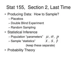
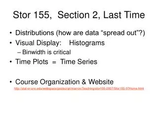
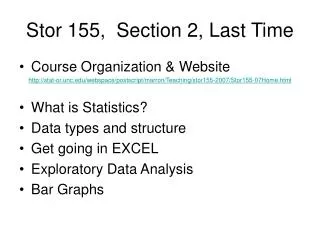
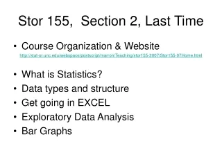
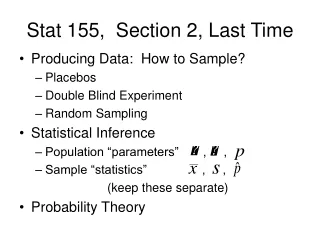
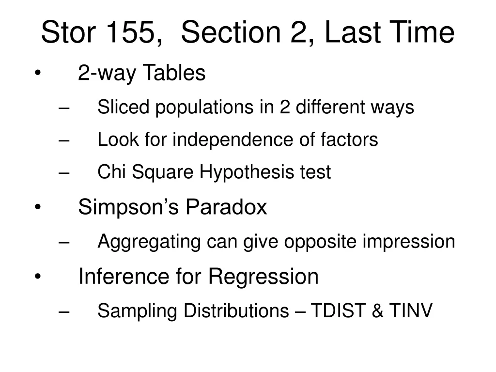
Stor 155, Section 2, Last Time • 2-way Tables • Sliced populations in 2 different ways • Look for independence of factors • Chi Square Hypothesis test • Simpson’s Paradox • Aggregating can give opposite impression • Inference for Regression • Sampling Distributions – TDIST & TINV
Reading In Textbook Approximate Reading for Today’s Material: Pages 634-667 & Review Approximate Reading for Next Class: Pages 634-667 & Review
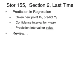
Inference for Regression Chapter 10 Recall: • Scatterplots • Fitting Lines to Data Now study statistical inference associated with fit lines E.g. When is slope statistically significant?
Recall Scatterplot For data (x,y) View by plot: (1,2) (3,1) (-1,0) (2,-1)
Recall Linear Regression Idea: Fit a line to data in a scatterplot • To learn about “basic structure” • To “model data” • To provide “prediction of new values”
Recall Linear Regression Given a line, , “indexed” by Define “residuals” = “data Y” – “Y on line” = Now choose to make these “small”
Recall Linear Regression Make Residuals > 0, by squaring Least Squares: adjust to Minimize the “Sum of Squared Errors”
Least Squares in Excel Computation: • INTERCEPT (computes y-intercept a) • SLOPE (computes slope b) Revisit Class Example 14 http://stat-or.unc.edu/webspace/postscript/marron/Teaching/stor155-2007/Stor155Eg14.xls
Inference for Regression Idea: do statistical inference on: • Slope a • Intercept b Model: Assume: are random, independent and
Inference for Regression Viewpoint: Data generated as: y = ax + b Yi chosen from Xi Note: a and b are “parameters”
Inference for Regression Parameters and determine the underlying model (distribution) Estimate with the Least Squares Estimates: and (Using SLOPE and INTERCEPT in Excel, based on data)
Inference for Regression Distributions of and ? Under the above assumptions, the sampling distributions are: • Centerpoints are right (unbiased) • Spreads are more complicated
Inference for Regression Formula for SD of : • Big (small) for big (small, resp.) • Accurate data Accurate est. of slope • Small for x’s more spread out • Data more spread More accurate • Small for more data • More data More accuracy
Inference for Regression Formula for SD of : • Big (small) for big (small, resp.) • Accurate data Accur’te est. of intercept • Smaller for • Centered data More accurate intercept • Smaller for more data • More data More accuracy
Inference for Regression One more detail: Need to estimate using data For this use: • Similar to earlier sd estimate, • Except variation is about fit line • is similar to from before
Inference for Regression Now for Probability Distributions, Since are estimating by Use TDIST and TINV With degrees of freedom =
Inference for Regression Convenient Packaged Analysis in Excel: Tools Data Analysis Regression Illustrate application using: Class Example 32, Old Text Problem 10.12
Inference for Regression Class Example 32, Old Text Problem 10.12 Utility companies estimate energy used by their customers. Natural gas consumption depends on temperature. A study recorded average daily gas consumption y (100s of cubic feet) for each month. The explanatory variable x is the average number of heating degree days for that month. Data for October through June are:
Inference for Regression Data for October through June are:
Inference for Regression Class Example 32, Old Text Problem 10.12 Excel Analysis: http://stat-or.unc.edu/webspace/postscript/marron/Teaching/stor155-2007/Stor155Eg32.xls Good News: Lots of things done automatically Bad News: Different language, so need careful interpretation
Inference for Regression Excel Glossary:
Inference for Regression Excel Glossary:
Inference for Regression Excel Glossary:
Inference for Regression Excel Glossary:
Inference for Regression Some useful variations: Class Example 33, Text Problems 10.23 - 10.25 Excel Analysis: http://stat-or.unc.edu/webspace/postscript/marron/Teaching/stor155-2007/Stor155Eg33.xls
Inference for Regression Class Example 33, (10.23 – 10.25) Engineers made measurements of the Leaning Tower of Pisa over the years 1975 – 1987. “Lean” is the difference between a points position if the tower were straight, and its actual position, in tenths of a meter, in excess of 2.9 meters. The data are:
Inference for Regression Class Example 33, (10.23 – 10.25) The data are:
Inference for Regression Class Example 33, (10.23 – 10.25) : • Plot the data, does the trend in lean over time appear to be linear? • What is the equation of the least squares fit line? • Give a 95% confidence interval for the average rate of change of the lean. http://stat-or.unc.edu/webspace/postscript/marron/Teaching/stor155-2007/Stor155Eg33.xls
Inference for Regression HW: 10.17 b,c 10.26 (using log base 10, for part c: Est’d slope: 0.194 Est'd intercept: -379 95% CI for slope: [0.186, 0.202])
And Now for Something Completely Different Graphical Displays: • Important Topic in Statistics • Has large impact • Need to think carefully to do this • Watch for attempts to fool you
And Now for Something Completely Different Graphical Displays: Interesting Article: “How to Display Data Badly” Howard Wainer The American Statistician, 38, 137-147. Internet Available: http://links.jstor.org
And Now for Something Completely Different Main Idea: • Point out 12 types of bad displays • With reasons behind • Here are some favorites…
And Now for Something Completely Different Hiding the data in the scale
And Now for Something Completely Different The eye perceives areas as “size”:
And Now for Something Completely Different Change of Scales in Mid-Axis Really trust the Post???
Review Slippery Issues Major Confusion: Population Quantities Vs. Sample Quantities
Review Slippery Issues Population Quantities: • Parameters • Will never know • But can think about Sample Quantities: • Estimates (of parameters) • Numbers we work with • Contain info about parameters
Review Slippery Issues Population Mathematical Notation: (fixed & unknown) Sample Mathematical Notation : (summaries of data, have numbers)
Review Slippery Issues Sampling Distributions: Measurement Error: Counting / Proportions:
Review Slippery Issues Confidence Intervals: Based on margin of error: Measurement Error: brackets 95% of time Counting / Proportions: brackets 95% of time
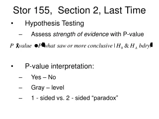
Review Slippery Issues Hypothesis Testing: Statement of Hypotheses: Actual Test: P-value = P{What saw or m.c. | Bdry}
Hypothesis Testing from 3/22 Other views of hypothesis testing: View 2: Z-scores Idea: instead of reporting p-value (to assess statistical significance) Report the Z-score A different way of measuring significance
Hypothesis Testing – Z scores E.g. Fast Food Menus: Test Using P-value = P{what saw or m.c.| H0 & HA bd’ry}
Hypothesis Testing – Z scores P-value = P{what saw or or m.c.| H0 & HA bd’ry}