Rendering Overview
Rendering Overview. CSE 3541 Matt Boggus. Rendering. Algorithmically generating a 2D image from 3D models Raster graphics. CSE OSU rendering courses. CSE 5542 Real Time Rendering

Rendering Overview
E N D
Presentation Transcript
Rendering Overview CSE 3541 Matt Boggus
Rendering • Algorithmically generating a 2D image from 3D models • Raster graphics
CSE OSU rendering courses • CSE 5542 Real Time Rendering • Comprehensive list of topics in real-time rendering using OpenGL and GLSL, including coordinate systems, transformations, viewing, illumination, texture mapping, and shader-based algorithms. • CSE 5545 Advanced Computer Graphics • Advanced topics in computer graphics; image synthesis, lighting and rendering, sampling and material properties, volume rendering.
Topics • Lighting models and shading • Viewing transformations • Raytracing overview
Physics of light Red lines – single bounce ; local illumination Green lines – multiple bounce ; global illumination
Point light Emit light in all directions Vector from point to light
Directional light Light vector always the same
Area light Requires sampling – pick point on the light then generate the vector from point on the surface to point on the light
Light scattering on a surface Figure from http://en.wikipedia.org/wiki/Bidirectional_scattering_distribution_function
Ambient illumination • Approximation for global illumination • Often set as a constant value, resulting in object having one, flat color • Lambient = Iambient * Kambient • [Light = Intensity * Material] • Notable exceptions: • Ambient occlusion • Radiant flux
Diffuse illumination • Diffuse reflection assumes that the light is equally reflected in every direction. • In other words, if the light source and the object has fixed positions in the world space, the camera motion doesn’t affect the appearance of the object. • The reflection only depends on the incoming direction. It is independent of the outgoing (viewing) direction.
Diffuse illumination • Ldiffuse = Idiffuse * Kdiffuse* cosθi
Specular illumination • Some materials, such as plastic and metal, can have shiny highlight spots. • This is due to a glossy mirror-like reflection. • Materials have different shininess/glossiness.
Specular reflection • R = 2(L⋅N)N- L • Lspecular= Ispecular * Kspecular * cosnφ • n is shininess coefficient • φ is the angle between EYE and R
Normal of vertex Average the normals of the polygons it is used in
Shading model comparison Flat shading – one normal per polygon Gouraud shading – one normal per vertex ; compute color of a point on the polygon by: computing color at each vertex and linearly interpolate colors inside the polygon Phong shading – one normal per vertex ; compute color of a point on the polygon by: linearly interpolate the normal vector, then perform lighting calculation
Viewing transformation parameters • Camera (eye) position (ex,ey,ez) • Center of interest (cx, cy, cz) • Or equivalently, a “viewing vector” to specify the direction the camera faces • Up vector (Up_x, Up_y, Up_z)
Eye coordinate system • Camera (eye) position (ex,ey,ez) • View vector : v • Up vector : u • Third vector (v x u) : w • Viewing transform – construct a matrix such that: • Camera is translated to the origin • Camera is rotated so that • v is aligned with (0,0,1) or (0,0,-1) • u is aligned with (0,1,0)
Projection • Transform a point from a high dimensionalspace to a low‐dimensional space. • In 3D, the projection means mapping a 3D point onto a 2D projection plane (or called image plane). • There are two basic projection types: • Parallel (orthographic) • Perspective
Properties of orthographic projection • Not realistic looking • Can preserve parallel lines • Can preserve ratios • Does not preserve angles between lines • Mostly used in computer aided design and architectural drawing software
Properties of perspective projection • Realistic looking • Lines are mapped to lines • Parallel lines may not remain parallel • Ratios are not preserved • Distances cannot be directly measured, as in parallel projection
Another use of perspective • Head Tracking for Desktop VR Displays using the WiiRemote
Ray Tracing • Algorithm: Shoot a ray through each pixel Find first object intersected by ray Image plane Eye • Computation: • Compute ray (orthographic or perspective?) • Compute ray-object intersections (parametric line equation) • Compute shading (use light and normal vectors)
Shade of Object at Point • Ambient • Diffuse • Specular • Texture • Shadows • Reflections • Transparency (refraction)
Shadows • Determine when light ray is blocked from reaching object. • Ray-object intersection calculation For each pixel for each object for each light source for each object
Eye Reflection Image plane
Transparency & Refraction • Ray changes direction in transition between materials • Material properties give ratio of in/out angles
Eye Recursive Ray Tracing Image plane
Sampling and Aliasing Problem: Representing pixel by a single ray.
Efficiency • 1280 x 1024 = 1,310,720 106 pixels. • 106 initial rays. • 106 reflection rays. • Potentially 106 refraction rays. • 3 x 10⁶ shadow rays (3 lights.) Next level: • Potentially 4 x 10⁶ refraction/reflection rays. 1,000,000 polygons. 107 x 106 = 1013 ray-polygon intersection calculations.
Intersection Data Structures Coarse test to see if a ray could *possibly* intersect object OR Divide space up – sort objects into spatial buckets – trace ray from bucket to bucket