Download
1 / 14
140 likes | 257 Views
These are the wave function solutions ( eigenfunctions ) for the finite square well. These are the 4 equations from applying the continuity of psi and its first derivative at the well boundaries. Now add (1) and (3). S ubtract (3) from (1). Now add (2) and (4). S ubtract (4) from (2).

E N D
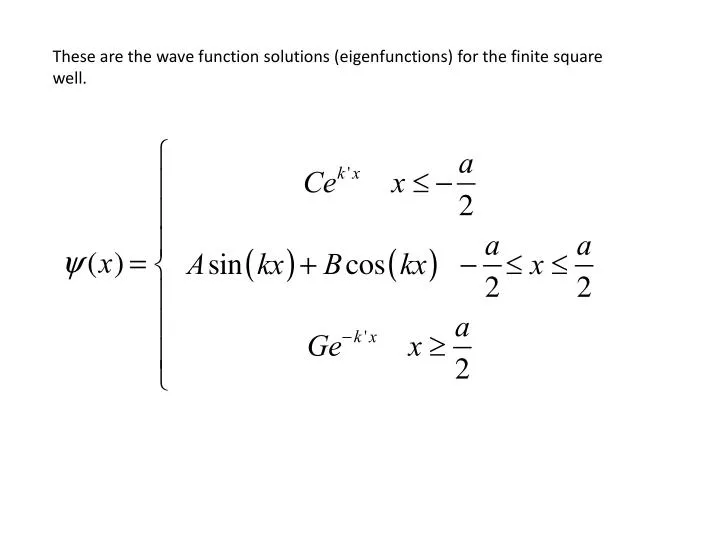
These are the wave function solutions (eigenfunctions) for the finite square well.
These are the 4 equations from applying the continuity of psi and its first derivative at the well boundaries.
Now add (1) and (3) Subtract (3) from (1) Now add (2) and (4) Subtract (4) from (2)
As long as and divide (8) by (5) As long as and divide (6) by (7)
Both (9) and (10) cannot both be true at the same time. Proof: add the two equations Which cannot be since both k and a are real.
Solutions of the second kind: odd solutions Solutions of the first kind: Even solutions From the even solutions, we have that: So it must be the case for the even solutions that:
Using these relations below we can write the wave functions for the square well – even solutions.
Using one of the boundary conditions we can solve for B And the wave functions (Eigenfunctions) in each region are (where B is determined by normalization in each region so to match the solutions at the boundaries.)
Let’s look at the even solutions and determine the allowed energies
The tangent term as an a/2 factor. Let’s put that in everything. Define alpha and r as:
A special case: the infinite square well: Which are half of the allowed energy states of the infinite square well (n odd).
Let’s go back and find the solutions for the allowed energies by graphing P(a) Q(a) This cannot be solved analytically. So, where the two functions these will be related to the allowed energies for the case of r = 2 as an example.
From Mathematica we can find the places where these two functions cross. They are given by x below which is what we’ve called alpha: FindRoot[p[x] == q[x], {x, 1.2}] {x -> 1.25235} FindRoot[p[x] == q[x], {x, 3.6}] {x -> 3.5953} Now to calculate the values of the allowed energies.
continuum V0 E3=0.808V0 E3=0.383V0 E3=0.098V0