Download

1 / 27
410 likes | 916 Views
Lecture 5. Application of GNSS in Surveying. Contents. Absolute vs. Relative positioning Applications in Surveying static vs. kinematic positioning The GNSS infrastructure and its evolution Transformation of WGS-84 coordinates to the national coordinate system. Absolute positioning.

E N D
Lecture 5. Application of GNSS in Surveying
Contents • Absolute vs. Relative positioning • Applications in Surveying • static vs. kinematic positioning • The GNSS infrastructure and its evolution • Transformation of WGS-84 coordinates to the national coordinate system
Absolute positioning All systematic error sources should be modelled (limited accuracy)
Relative positioning • Eliminates (or reduces) the effect of error sources, like: • orbit and clock error; • ionospheric error (for short baselines)
Static GPS observations • Static GPS Observations • At least two receivers • The base station is set up on a control point (known coordinates) • The rover station is set up on an unknown point. • same receiver configuration of base and rover (obs. interval, elevation mask) • Time span: • 1 freq.: 30 min+ 5min/km (up to 10 km) • 2 freq: 20 Min + 5 Min/km • Accuracy: 1 cm or better (for longer observations even 1-2 mm in a distance of 15km)
Kinematic observations • Kinematic observations • At least two receivers • Base receiver on a control point • Rover station must be initialized (at least 20 Min on the same Point) • Afterwards the rover can survey the points. • time span: 5-10 secs per point
Kinematic obs. with OTF initialization OTF (on-the-fly) initialization
Real-time kinematic observations Pi– pseudorange observation; Yi – phase range observation
Real-time kinematic observations • Real-Time Kinematic Observations • At least two receivers (preferably 2 freq.) • Base on a control point. • Real time data broadcasting (phase observations and base coordinates) between base and rover (radio, GSM, internet) • Ca 1-5 min to determine the ambiguity parameters • after the solution of the ambiguity parameters, the unknown points can be measured. • time span: 2-3 sec perpoint
Post-processing vs real-time • Post processing: (observations are processed in the office) • static observations; • kinematic observations; • Real-time: (observations are processed on-site) • real time kinematic.
Network observations Radial configuration Network configuration
Point reconnaissance • How should the place of the points be selected? • a clear view to the sky; • free of electromagnetic interference (no high voltage wires in the vicinity); • the point should be in public area, close to roads; • the stability of the points should be ensured. The selected stations should be marked, the position of the obstructing objects should be noted
Planning the observations • in case of obstructing objects, or high accuracy requirements, the observations can be planned; • planning software predicts the number of visible satellites, the PDOP values by knowing the approximate positions of the satellites and the approximate station coordinate. • The position of obstructed objects can be added to the planner software, thus the effect of the obstructed sky can be estimated. • Using the PDOP values, the suitable time window can be selected for the observations.
GNSS Infrastructure • Positioning in Surveying: • relative positioning can provide the sufficient accuracy; • base stations are required; • usually a base-rover pair is used for positioning, which is not effetive; • Solution: • continuously operating reference stations (CORS); • act as a base station, but broadcasts corrections to many rovers at the same time;
Generations of GNSS Infrastructure 1st Generation: Permanent stations, which log the received data for post processing only. Data can be downloaded from the internet, and rover observations can be processed with these downloaded data.
Generations of GNSS Infrastructure 2nd Generation: Permanent stations, which log the received data, but broadcast it in real-time, too. Data can be used for post processing and real-time application as well. Real-time kinematic positioning is achieved by a single base station. RTK (3 cm) up to 35 km from the reference stations (in case of 2 frequencies)
Generations of GNSS Infrastructure 3rd Generation: A network of permanent stations, which broadcasts the data to a processing facility. This facility monitors and models the systematic error of positioning (ionosphere, troposphere, orbit and clock error, etc.). These models are used for the positioning as well.
Augmentation Systems Ground based (GBAS): The GNSS Infrastructure, the network of continuously operating reference stations and the processing facility. The corrections are broadcasted through radiolink or the internet. Satellite based (SBAS): A network of ground based stations to monitor the systematic error sources, effects are modelled, and corrections are broadcasted to geostationary satellites, which transmit a GPS like signal to the GNSS receivers (EGNOS, WAAS, etc.)
Transforming the GPS coordinates • GPS observations refer to the WGS-84 coordinate system. • Local coordinate grids are linked with a local ellipsoid, which • usually not geocentric; • has different size than the WGS-84 ellipsoid. • a link should be established between the two systems to be able to compute the grid coordinates from the WGS-84 ones Coordinate Transformation
Transforming the GPS coordinates • Common points in both coordinate systems (local and WGS-84) are needed. • In rectangular coordinate systems the 3D Helmert-transformation can be used to compute the coordinates in the local system: • Where: • x,y,z are the local cartesian coordinates; • DX, DY, DZ are the elements of the translation vector; • X,Y,Z are the WGS-84 cartesian coordinates; • R is the rotation matrix; • m is the scale factor.