Download
1 / 53
530 likes | 810 Views
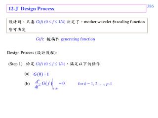
12-J Design Process. 設計時,只要 G ( f ) (0 f 1/4) 決定了, mother wavelet 和 scaling function 皆可決定. G ( f ) : 被稱作 generating function. Design Process ( 設計流程 ):. (Step 1): 給定 G ( f ) (0 f 1/4) ,滿足以下的條件. (a). (b). for k = 1, 2, …, p -1. (Step 2) 由.

E N D
12-J Design Process 設計時,只要 G(f) (0 f 1/4)決定了,mother wavelet 和scaling function 皆可決定 G(f): 被稱作generating function Design Process (設計流程): (Step 1): 給定 G(f) (0 f 1/4),滿足以下的條件 (a) (b) for k = 1, 2, …, p-1
(Step 2) 由 決定G(f) (3/4 f < 1) (Step 3) 由 決定G(f) (1/4 < f < 3/4) 再根據 G(f) = G(f+1),決定所有的 G(f) 值 (Step 4) 由 決定H(f) (Step 5) 由 決定(f), (f)
註: (1) 當 Step 1 的兩個條件滿足,由於 for k = 0, 1, 2, …, p-1 又由於 for k = 0, 1, 2, …, p-1 (2) 所以當 G(f) (0 f 1/4) 給定,|G(f)| 有唯一解
12-K Several Continuous Wavelets with Discrete Coefficients (1) Haar Wavelet g[0] = 1, g[1] = 1 h[0] = 1, h[1] = −1 或 g[0] = 1/2, g[1] = 1/2 h[0] = 1/2, h[1] = −1/2 vanish moment = ?
(2) Sinc Wavelet for |f | 1/4 otherwise vanish moment = ? (3) 4-point Daubechies Wavelet vanish moment = ? vanish moment VS the number of coefficients
From: S. Qian and D. Chen, Joint Time-Frequency Analysis: Methods and Applications, Prentice Hall, N.J., 1996.
12-L Continuous Wavelet with Discrete Coefficients 優缺點 Advantages: (1) Fast algorithm for MRA (2) Non-uniform frequency analysis FT (3) Orthogonal
Disadvantages: (a) 無限多項連乘 (b) problem of initial 皆由 算出 如何算 (c) 難以保證 compact support (d) 仍然太複雜
XIII. Discrete Wavelet Transform (DWT) 13.1 概念 (1) discrete input to discrete output (2) 由 continuous wavelet transform with discrete inputs 演變而來的,(比較 page 356)但是大幅簡化了其中的數學 (3) 忽略了 scaling function 和 mother wavelet function 的分析 但是保留了階層式的架構
13.2 1-D Discrete Wavelet Transform lowpass filter g[n] 2 x1,L[n] input L-points x[n] highpass filter N-points h[n] 2 x1,H[n] L-points 2 : downsampling by the factor of 2 x[n] z[n] Q
輸入: x[n] (不需算 , 直接以 x[n] 作為 initial Low pass filter g[n] High pass filter h[n] 角色似 scaling function 角色似 wavelet function (相當於 page 356 的 gn) (相當於 page 356 的 hn) 1st stage
further decomposition (from the (a−1)th stage to the ath stage) x2,L[n] g[n] 2 g[n] x1,L[n] 2 2 x2,H[n] h[n] x[n] x1,H[n] 2 h[n]
xa,H[n] (1) 有的時候,對於 也再作細分 (2) 若 input 的 x[n] 的 length 為N, 則 ath stage xa,L[n], xa,H[n] 的 length 為N/2a (3) 經過 DWT 之後,全部點數仍接近 N點
(4) 以頻譜來看 X1,L(f) X1,H(f) X1,H(f) X2,L(f) X2,H(f) X1,H(f) X2,H(f) X3,L(f) X3,H(f)
13.3 2-D Discrete Wavelet Transform g[m] 2 x1,L[m, n] along m g[n] 2 v1,L[m, n] along n h[m] 2 x1,H1[m, n] x[m, n] along m x1,H2[m, n] g[m] 2 h[n] 2 v1,H[m, n] along m along n 2 x1,H3[m, n] h[m] along m
輸入: x[m, n] Low pass filter g[n] High pass filter h[n] along n along m
n m x3,H3 x2,H3[m, n] 原圖:正方形 x1,H3[m, n] from R. C. Gonzalez and R. E. Woods, Digital Image Processing, Chap. 7, 2ndedition, Prentice Hall, New Jersey, 2002.
原圖:Lena from R. C. Gonzalez and R. E. Woods, Digital Image Processing, Chap. 7, 2ndedition, Prentice Hall, New Jersey, 2002.
compression & noise removing 保留 x1,L[m, n],捨棄其他部分 (directional) edge detection 保留 x1,H1[m, n] 捨棄其他部分 或保留 x1,H2[m, n] x1,H3[m, n] 當中所包含的資訊較少 corner detection?
13.4 Complexity of the DWT x[n] y[n], length(x[n]) = N, length(y[n]) = L, (N+L1)-point discrete Fourier transform (DFT) (N+L1)-point inverse discrete Fourier transform (IDFT) (1) Complexity of the 1-D DWT (without sectioned convolution)
(2) 當 N >>> L 時,使用 “sectioned convolution” 的技巧 x[n] x1[n] x2[n] x3[n] xS[n] n N1 N1 將 x[n] 切成很多段,每段長度為 N1 總共有 段 (N > N1 >> L)
complexity: 重要概念: The complexity of the 1-D DWT is linear with N when N >>> L
(3) Multiple stages 的情形下 若 xa,H[n] 不再分解 Complexity 近似於: 若 xa,H[n] 也細分 Complexity 近似於: (和 DFT 相近)
(4) Complexity of the 2-D DWT on page 400 (without sectioned convolution ) The first part needs M 1-D DWTs and the input for each 1-D DWT has N points The second part needs N+L1 1-D DWTs and the input for each 1-D DWT has M points
(5) Complexity of the 2-D DWT (with Sectioned Convolution) Image The original size: M N The size of each part: M1 N1 重要概念: If the method of the sectioned convolution is applied, the complexity of the 2-D DWT is linear with MN.
(6) Multiple stages, two dimension x[m, n] 的 size 為 M× N 若 xa,H1[n], xa,H2[n], xa,H3[n] 不細分,只細分 xa,L[n] total complexity 若 xa,H1[n], xa,H2[n], xa,H3[n] 也細分 total complexity
13.5 Many Operations Also Have Linear Complexities • 事實上,不只 wavelet 有 linear complexity 當 input 和 filter 長度或大小相差懸殊時 1-D convolution 的 complexity 是 linear with N. 2-D convolution 的 complexity 是 linear with MN. (和傳統 Nlog2N, MNlog2(MN) 的觀念不同) 很重要的概念
注意:DCT 的 complexity 也是 linear with MN (切成8 × 8 方格) complexity :
13.6 Reconstruction analysis synthesis g[n] 2 x1,L[n] 2 g1[n] x[n] x0[n] h[n] 2 x1,H[n] 2 h1[n] g1[n], h1[n] 要滿足什麼條件,才可以使得 x0[n] = x[n]? 2 : upsampling by the factor of 2 a[n] Q b[n] for r = 1, 2, Q−1
Reconstruction Problem 用 Z transform來分析
Z transform If a[n] = b[2n], (Proof): If a[2n] = b[n], a[2n+1] = 0
Perfect reconstruction: 條件: where
13.7 Reconstruction 的等效條件 if and only if 這四個條件被稱作 biorthogonal conditions
(Proof) Note: (a) (b) 令 Therefore, From inverse Z transform
orthogonality 條件 1 (c) Similarly, substitute into after the process the same as that of the above orthogonality 條件 2
(d) Since orthogonality 條件 3 (e) 同理 orthogonality 條件 4
13.8 DWT 設計上的條件 Reconstruction Finite length 為了 implementation 速度的考量 g[n] 0 only when L n L h[n] 0 only when L n L h1[n] , g1[n] ? 令 則根據 page 414, 複習:
因為 k必需為 odd Lowpass-highpass pair
整理:DWT 的四大條件 (1) (for reconstruction) (2) h[n] 0 only when L n L (h[n], g[n] have finite lengths) g[n] 0 only when L n L (3) k必需為 odd (h1[n], g1[n] have finite lengths) (4) h[n] 為 highpass filter (lowpass and highpass pair) g[n] 為 lowpass filter 第三個條件較難達成,是設計的核心
13.9 Two Types of Perfect Reconstruction Filters (1) QMF (quadrature mirror filter) k is odd g[n] has finite length
(2) Orthonormal k is odd g1[n] has finite length
大部分的 wavelet 屬於 orthonormal wavelet 文獻上,有時會出現另一種 perfect reconstruction filter, 稱作 CQF (conjugate quadrature filter) 然而,CQF 本質上和 orthonormal filter 相同
13.10 Several Types of Discrete Wavelets discrete Haar wavelet (最簡單的) otherwise otherwise otherwise otherwise 是一種 orthonormal filter
discrete Daubechies wavelet (8-point case) otherwise n = 0 ~ 7 n = 0 ~ 7 otherwise n = −7 ~ 0 otherwise otherwise n = −7 ~ 0
discrete Daubechies wavelet (4-point case) discrete Daubechies wavelet (6-point case) discrete Daubechies wavelet (10-point case) discrete Daubechies wavelet (12-point case)
symlet (6-point case) symlet (8-point case) symlet (10-point case) Daubechies wavelets and symlets are defined for N is a multiple of 2
coilet (6-point case) coilet (12-point case) Coilets are defined for N is a multiple of 6 The Daubechies wavelet, the symlet, and the coilet are all orthonormal filters.
The Daubechies wavelet, the symlet, and the coilet are all derived from the “continuous wavelet with discrete coefficients” case. Physical meanings: • Daubechies wavelet The ? point Daubechies wavelet has the vanish moment of p. • Symlet The vanish moment is the same as that of the Daubechies wavelet, but the filter is more symmetric. • Coilet The scaling function also has the vanish moment. for 1 ≦ k ≦ p
附錄十三 誤差計算的標準 若原來的信號是 x[m, n],要計算 y[m, n] 和 x[m, n] 之間的誤差,有下列幾種常見的標準 (1) maximal error (2) square error (3) error norm (i.e., Euclidean distance) (4) mean square error (MSE),信號處理和影像處理常用