Download
1 / 47
470 likes | 627 Views
Using polynomials and matrix splittings to sample from LARGE Gaussians. Al Parker and Colin Fox SUQ13 June 4, 2013. Outline. Iterative linear solvers and Gaussian samplers … Convergence theory is the same Same reduction in error per iteration A sampler stopping criterion

E N D
Using polynomials and matrix splittings to sample from LARGE Gaussians Al Parker and Colin Fox SUQ13 June 4, 2013
Outline • Iterative linear solvers and Gaussian samplers … • Convergence theory is the same • Same reduction in error per iteration • A sampler stopping criterion • How many sampler iterations to convergence? • Samplers equivalent in infinite precision perform differently in finite precision. • State of the art: CG-Chebyshev-SSOR Gaussian sampler • In finite precision, convergence to N(0, A-1) implies convergence to N(0,A). The converse is not true. • Some future work
Correspondence between solvers and samplers of N(0, A-1) Solving Ax=b: Gauss-Seidel Chebyshev-GS CG Sampling y ~ N(0,A-1): Gibbs Chebyshev-Gibbs CG-Lanczos sampler
We consider iterative solvers of Ax = b of the form: 1. Split the coefficient matrix A = M - N for M invertible. 2.xk+1 = (1- vk) xk-1 + vkxk + vkuk M-1 (b-A xk) for some parametersvkand uk. 3. Check for convergence: Quit if ||b - A xk+1 || is small. Otherwise, update vkand uk, go to step 2. Need to be able to inexpensively solve M u = r Given M, it’s the same cost per iteration regardless of acceleration method used
For example … xk+1 = (1- vk) xk-1 + vkxk + vkuk M-1 (b-A xk) Chebyshev-GS CG Gauss-Seidel M = MGS D MTGS, vkand ukare functions of the 2 extreme eigenvalues of I - G=M-1A M = I, vk , ukare functions of the residuals b - Axk MGS = D + L, vk = uk = 1
... and the solver error decreases according to a polynomial, (xk- A-1b) = Pk(I-G)(x0 - A-1b), G=M-1NI – G = M-1A CG Gauss-Seidel Chebyshev-GS Pk(I-G) is the kth order Chebyshev polynomial (the polynomial with smallest maximum between the two eigenvalues of I - G). Pk(I-G) = Gk Pk(I-G) is the kth order Lanczospolynomial
... and the solver error decreases according to a polynomial, (xk- A-1b) = Pk(I-G)(x0 - A-1b), G=M-1NI – G = M-1A CG Gauss-Seidel Chebyshev-GS Pk(I-G) the kth order Chebyshev polynomial, asymptotic average reduction factor is optimal, Pk(I-G) = Gk, stationary reduction factor is Pk(I-G) is the kth order Lanczospolynomial converges in a finite number of steps* depending on eig(I-G) p(G)
Some common iterative linear solvers CG is guaranteed to accelerate * Chebyshev is guaranteed to accelerate*
Iterative linear solver performance in finite precision • Table from Fox & P, in prep. • Ax = b was solved for SPD 100 x 100 first order locally linear sparse matrix A. • Stopping criterion was ||b - A xk+1 ||2 < 10-8.
Iterative linear solver performance in finite precision p(G)
What iterative samplers of N(0, A-1) are available? Solving Ax=b: Gauss-Seidel Chebyshev-GS CG Sampling y ~ N(0,A-1): Gibbs Chebyshev-Gibbs CG-Lanczos sampler
We study iterative samplers of N(0, A-1) of the form: 1. Split the precision matrix A = M - N for M invertible. 2. Sample ck ~ N(0, (2-vk)/vk ( (2 – uk)/ ukMT + N) 3. yk+1 = (1- vk) yk-1 + vkyk + vkuk M-1 (ck -A yk). 4. Check for convergence: Quit if “the difference” between N(0, Var(yk+1)) and N(0, A-1) is small. Otherwise, update linear solver parameters vkand uk, go to step 2. Need to be able to inexpensively solve M u = r Need to be able to easily sample ck Given M, it’s the same cost per iteration regardless of acceleration method used
For example … yk+1 = (1- vk) yk-1 + vkyk + vkuk M-1 (ck -A yk) ck ~ N(0, (2-vk)/vk ( (2 – uk)/ ukMT + N) Gibbs Chebyshev-Gibbs CG-Lanczos M = MGS D MTGS, vkand ukare functions of the 2 extreme eigenvalues of I-G=M-1A M = I, vk , ukare functions of the residuals b - Axk MGS = D + L, vk = uk = 1
... and the sampler error decreases according to a polynomial, (A-1 - Var(yk))v = 0 for any Krylov vector v (E(yk) - 0)=Pk(I-G)(E(y0) – 0) (A-1 - Var(yk)) = Pk(I-G)(A-1 - Var(y0))Pk(I-G)T CG-Lanczos Gibbs Chebyshev-Gibbs Pk(I-G) kth order Chebyshevpolyomial, optimal asymptotic average reduction factor is Pk(I-G) = Gk, with error reduction factor Var(yk) is the kth order CG polynomial converges in a finite number of steps* in a Krylov space depending on eig(I-G) p(G)2
My attempt at the historical development of iterative Gaussian samplers:
Theorem An iterative Gaussian sampler converges (to N(0, A-1)) faster # than the corresponding linear solver as long as vk , ukare independent of the iterates yk(Fox & P 2013). Gibbs Sampler Chebyshev Accelerated Gibbs
Theorem An iterative Gaussian sampler converges (to N(0, A-1)) faster# than the corresponding linear solver as long as vk , ukare independent of the iterates yk(Fox & P 2013). # The sampler variance error reduction factor is the square of the reduction factor for the solver: So: • The Theorem does not apply to Krylov samplers. • Samplers can use the same stopping criteria as solvers. • If a solver converges in n iterations, so does the sampler Stationary sampler: p(G)2
In theory and finite precision, • Chebyshev acceleration is faster than a Gibbs sampler Example: N(0, -1 ) in 100D Covariance matrix convergence, ||A-1 – Var(yk)||2 /||A-1 ||2 Benchmark for cost in finite precision is the cost of a Cholesky factorization Benchmark for convergence in finite precision is 105Cholesky samples
Algorithm for an iterative sampler of N(0, A-1) with a vague stopping criterion: 1. SplitA = M - N for M invertible. 2. Sample ck ~ N(0, (2-vk)/vk ( (2 – uk)/ ukMT + N) 3. yk+1 = (1- vk) yk-1 + vkyk + vkuk M-1 (ck -A yk). 4. Check for convergence: Quit if “the difference” between N(0, Var(yk+1)) and N(0, A-1) is small. Otherwise, update linear solver parameters vkand uk, go to step 2.
Algorithm for an iterative sampler of N(0, A-1) with an explicit stopping criterion: 1. SplitA = M - N for M invertible. 2. Sample ck ~ N(0, (2-vk)/vk ( (2 – uk)/ ukM + N) 3. xk+1 = (1- vk) xk-1 + vkxk + vkuk M-1 (b-Axk) 4. yk+1 = (1- vk) yk-1 + vkyk + vkuk M-1 (ck -Ayk) 5. Check for convergence: Quit if ||b - A xk+1 || is small. Otherwise, update linear solver parameters vkand uk, go to step 2.
An example: a Gibbs sampler of N(0, A-1) with a stopping criterion: 1. SplitA = M - N where M = D + L 2. Sample ck ~ N(0, MT + N) 3. xk+1 = xk + M-1 (b - A xk) <------ Gauss-Seidel iteration 4. yk+1 = yk + M-1 (ck -A yk) <------ (bog standard) Gibbs iteration 5. Check for convergence: Quit if ||b - A xk+1 || is small. Otherwise, go to step 2.
Stopping criterion for the CG sampler • The CG sampler also uses ||b - A xk+1 || as a stopping criterion, but a small residual merely indicates that the sampler has successfully sampled (i.e., ‘converged’) • in a Krylov subspace • (this same issue occurs with CG-Lanczos solvers). Only 8 eigenvectors (corresponding to the 8 largest eigenvalues of A-1) are sampled by the CG sampler
Stopping criteria for the CG sampler • The CG sampler also uses ||b - A xk+1 || as a stopping criterion, but a small residual merely indicates that the sampler has successfully sampled (i.e., ‘converged’) • in a Krylov subspace • (this same issue occurs with CG-Lanczos solvers). • A coarse assessment of the accuracy of the distribution of the CG sample is to estimate (P & Fox 2012): • trace(Var(yk))/trace(A-1 ). • The denominator trace(A-1 ) is estimated by the CG sampler using a sweet-as (minimum variance) Lanczos Monte Carlo scheme (Bai, Fahey, & Golub 1996).
Example: 102Laplacian over a 10x10 2D domain eigenvalues of A-1 37 eigenvectors are sampled (and estimated) by the CG sampler. A=
A priori calculation of the number of solveriterations to convergence Since the solver error decreases according to a polynomial, (xk- A-1b) = Pk(I-G)(x0 - A-1b), G=M-1N • then the estimated number of iterations k until the error reduction||xk- A-1b|| / ||x0 - A-1b <ε is about (Axelsson 1996): • Stationary splitting: • k = lnε/ ln(p(G)) • Chebyshev: • k = ln(ε/2)/lnσ Gauss-Seidel Chebyshev-GS Pk(I-G) is the kth order Chebyshev polynomial Pk(I-G) = Gk
A priori calculation of the number of sampleriterations to convergence ... and since the sampler error decreases according to the same polynomial (E(yk) – 0)=Pk(I-G)(E(y0) – 0) • (A-1 - Var(yk)) = Pk(I-G)(A-1 - Var(y0))Pk(I-G)T Gibbs Chebyshev-Gibbs Pk(I-G) is the kth order Chebyshev polynomial Pk(I-G) = Gk
A priori calculation of the number of sampleriterations to convergence ... and since the sampler error decreases according to the same polynomial (E(yk) – 0)=Pk(I-G)(E(y0) – 0) • (A-1 - Var(yk)) = Pk(I-G)(A-1 - Var(y0))Pk(I-G)T • THEN (Fox & Parker 2013) the suggested number of iterations k until the • error reduction • ||Var(yk) - A-1|| / ||Var(y0 ) - A-1|| < ε • is about: • Stationary splitting: k = lnε/ ln(p(G)2) • Chebyshev: k = ln(ε/2)/ln(σ2),
A priori calculation of the number of sampleriterations to convergence For example: Sampling from N(0, -1) Predicted vs. Actual number of iterations k until the error reduction in variance is less than ε = 10-8: p(G) = 0.9987, σ = 0.9312, Finite precision benchmark is the Cholesky relative error = 0.0525
“Equivalent” sampler implementations yield different results in finite precision
Different Lanczos sampling results due to different finite precision implementations • It is well known that “equivalent” • CG andLanczos algorithms (in exact arithmetic) perform • very differently in finite precision. • Iterative Krylov samplers • (i.e., with Lanczos-CD, CD, CG, orLanczos-vectors)are equivalent in exact arithmetic, but implementations in finite precision can yield different results. This is currently under numerical investigation.
Different Chebyshev sampling results due to different finite precision implementations • There are at least three implementations of modern (i.e., second-order) Chebyshev accelerated linear solvers • (e.g., Axelsson 1991, Saad 2003, and Golub & Van Loan 1996). • Some preliminary results comparing Axelsson and Saad implementations:
A fast iterative sampler (i.e., PCG-Chebyshev-SSOR) of N(0, A-1) (given a precision matrix A)
A fast iterative sampler for LARGE N(0, A-1): Use a combination of samplers: • Use a PCG sampler (with splitting/preconditionerMSSOR) to generate a sampleykPCGapprox. dist. asN(0, MSSOR1/2 A-1 MSSOR1/2) and estimates of the extreme eigenvaluesof I – G = MSSOR-1A. • Seed the samplesMSSOR-1/2 ykPCGand the extreme eigenvalues into a Chebyshev accelerated SSOR sampler. A similar to approach has been used running Chebyshev-accelerated solvers with multiple RHSs (Golub, Ruiz & Touhami 2007).
Example sampling via Chebyshev-SSOR sampling • from N(0, -1 ) in 100D Covariance matrix convergence, ||A-1 – Var(yk)||2 /||A-1 ||2
Comparing CG-Chebyshev-SSORto Chebyshev-SSOR sampling from N(0, ): Numerical examples suggest that seeding Chebyshev with a CG sample AND CG-estimated eigenvalues do at least as good a job as when using a “direct” eigen-solver (such as the QR-algorithm implemented via MATLAB’s eig( )).
Convergence to N(0, A-1) implies convergence to N(0,A). The converse is not necessarily true.
Can N(0, A-1) be used to sample from N(0,A)? • If you have an “exact” sample y ~ N(0, A-1), then simply multiplying by A yields a sample b = Ay ~ y ~ N(0, AA-1A) = N(0, A). • This result holds as long as you know how to multiply by A. • Theoretical support: • For a sample yk produced by the non-Krylov iterative samplers presented, the error in covariance of Ayk is: • A - Var(Ayk) = APk(I-G)(A- Var(Ay0)) Pk(I-G)T A • = Pk(I-GT)(A- Var(Ay0)) Pk(I-GT) T • Therefore, the asymptotic reduction factors of the stationary and Chebyshev samples of either ykorAyk are the same (i.e., p(G)2 and • resp.). • Unfortunately, whereas the reduction factor σ2 for Chebyshev sampling • yk~ N(0, A-1) is optimal, σ2 is (likely) less than optimal for Ayk ~ N(0, A).
Example of convergence using samples • yk~N(0, A-1) to generate samples • Ayk ~ N(0, A) A =
How about using N(0,A) to sample from N(0,A-1)? • You may have an “exact” sample • b ~ N(0, A) and yet you want y ~ N(0, A-1)(e.g., when studying spatiotemporal • patterns in tropical surface winds in Wikle et al. 2001). • Given b ~ N(0, A), then simply multiplying by A-1 yields a sample • y = A-1b ~ N(0, A-1AA-1) = N(0, A-1). • This result holds as long as you know how to multiply by A-1. • Unfortunately, it is often the case that multiplication by A-1 can only be performed approximately (e.g., using CG (Wikle et al. 2001)). • When using the CG solver to generate a sample ykCG ~= A-1 b when b ~ N(0,A), ykCGapprox. A-1 b gets ``stuck” in a k-dimensional Krylov subspace and only has the correct N(0, A-1) distribution if the k-dimensional Krylov space well approximates the eigenspaces corresponding to the large eigenvalues of of A-1 (P & Fox 2012). • Point: For large problems where direct methods are not available, use a Chebyshev accelerated solver to solve Ay = b to generate y ~ N(0, A-1) from b ~ N(0,A)!
Some Future Work • Meld a Krylov sampler (fast but “stuck” in a Krylov space in finite precision) with Chebyshev acceleration (slower but with guaranteed convergence). • Prove convergence of the Chebyshev accelerated sampler under • positivity constraints. • Apply some of these ideas to confocal microscope image analysis and nuclear magnetic resonance experimental designbiofilm problems.