Download
1 / 11
110 likes | 139 Views
Explore methods like Left-hand, Right-hand, and Midpoint Rectangular Approximation to estimate area under curves. Understand how distance equals area under velocity curve by considering a train moving steadily at 75 miles per hour. Practice estimating areas with multiple subintervals for better accuracy. Learn the Rectangular Approximation Method and different approaches to approximate areas.

E N D
A train moves along a track at a steady rate of 75 miles per hour from 7:00 am to 9:00 am. What is the total distance traveled by the train? • Answer: 150 miles • What would the graph of the velocity of this train look like?
velocity • time • Consider an object moving at a constant rate of 3 ft/sec. • Since rate . time = distance: • If we draw a graph of the velocity, the distance that the object travels is equal to the area under the line. • After 4 seconds, the object has gone 12 feet.
What if the velocity did not remain constant? • The graph would no longer be a straight line… • We can conclude from the two previous examples that the distance traveled by the object would still equal the area of the region under the velocity curve.
Consider a non-linear velocity curve… If the strips are narrow enough, they would be almost indistinguishable from rectangles. To find the area under the curve, we could add up all the individual rectangular areas. This is called RAM: Rectangular Approximation Method.
Approximate area: Let’s consider an actual function. • Example: • We could estimate the area under the curve by drawing rectangles touching at their left corners. • This is called the Left-hand Rectangular Approximation Method (LRAM).
Approximate area: • We could also use a Right-hand Rectangular Approximation Method (RRAM).
Approximate area: • Another approach would be to use rectangles that touch at the midpoint. This is the Midpoint Rectangular Approximation Method (MRAM). • In this example there are four subintervals. • As the number of subintervals increases, so does the accuracy.
The exact answer for this • problem is . • With 8 subintervals:
Find the LRAM, MRAM, and RRAM approximations to the area under the graph of y=x2 from x=0 to x=3 using six rectangles