Download
1 / 38
380 likes | 523 Views
3D Model Acquisition by Tracking 2D Wireframes. Presenter: Jing Han Shiau M. Brown, T. Drummond and R. Cipolla Department of Engineering University of Cambridge. Motivation. 3D models are needed in graphics, reverse engineering and model-based tracking.

E N D
3D Model Acquisition by Tracking 2D Wireframes Presenter: Jing Han Shiau M. Brown, T. Drummond and R. Cipolla Department of Engineering University of Cambridge
Motivation • 3D models are needed in graphics, reverse engineering and model-based tracking. • Want to be able to do real-time tracking.
Other Approaches • Optical flow/ structure from motion (Tomasi & Kanade, 1992) - Acquire a dense set of depth measurements - Batch method: not real-time • Point matching between images. - Feature extraction followed by geometric constraint enforcement • Edge extraction followed by line matching between 3 views using trifocal tensors
Improvement • Previous approaches used single line segments, but 2D wireframes allow high level user constraints to reduce the number of degrees of freedom (6 degree of freedom Euclidean motion constraint) since each new line segment adds 4 degrees of freedom.
3D Positions of Lines • Internal Camera parameters are known. • Initial and final camera matrices are known through querying robot (arm) for camera pose. • Edge correspondence preserved using tracking. • 3D position of lines computed by triangulation.
Single Line Tracking • Sample points are initialized along each line segment. • Search perpendicular to the line for local maxima of the intensity gradient. • New line position is chosen to minimize the sum squared distance to the measured edge positions.
Triangulation (Single Line tracking) • Finding 3D line by intersecting the rays corresponding to the ends of the line in the first image with the plane defined by the line in the second image.
Finding 3D Line • Find the 3D line by intersecting the world line defined by the point (u, v) in the first image, with the world plane defined by the line in the second, is equivalent to solving the linear equations
Limitations • Object edges which project to epipolar lines may not be tracked. In case of a pure camera translation, epipolar lines move parallel to themselves (radially with respect to the epipole); but the component of a line’s motion parallel to itself is not observable locally.
2D Wireframe Tracking • Similar to line segment tracking, least squares method is used to minimize the sum of the squared edge measurements from the wireframe.
2D Wireframe Tracking • The vertex image motions are stacked into the P-dimensional vector p, and the measurements are stacked into the D-dimensional vector d0. • D is the new measurement vector due to the motion p, and M is the DxP measurement matrix. • Least squares is used to minimize the sum squared measurement error |d|2.
2D Wireframe Tracking • The least squares solution is: • But in general it is not unique. It can contain arbitrary components in the right nullspace of M, corresponding to displacements of the vertex image positions that do not change the measurements. Adding a small constant to the diagonal of M prevents instability.
3D Model Building • 2D wireframe tracking preserves point correspondence. • 3D position of the vertices can be calculated from 2 views using triangulation. • Observations from multiple views can be combined by maintaining a 3D pdf for each vertex p(X). 3D pdf is updated on the basis of the tracked image position of the point, and the known camera.
3D Model Building • A 3D pdf has surfaces of constant probability defined by rays through a circle in the image plane. This pdf is approximated as a 3D Gaussian of infinite variance in the direction of the ray through the image point, and equal, finit, variance in the perpendicular plane.
3D Model Building • The 3D pdf is the likelihood of the tracked point position, conditioned on the current 3D position estimate –p(w|X). • Multiply this by the prior pdf to get the posterior pdf:
3D Model Building • X is Gaussian with mean mp and covariance matrix Cp, w|X is Gaussian with mean ml, covariance matrix Cl, and X|w is Gaussian with mean m and covariance matrix C. • These are the Kalman filter equations used to maintain 3D pdfs for each point.
Triangulation (3D Model Building) • Instead of using multiple rays that pass through the image point as in the case of single line tracking, probability distributionis used.
Combining Tracking and Model Building • There are 6 degrees of freedom corresponding to Euclidean position in space (3 translations and 3 rotations) for a rigid body. • A wireframe of P/2 points has a P-dimensional vector of vertex image positions.
Model-based 2D Tracking • The velocity of an image point for a normalized camera moving with translational velocity U and rotating with angular velocity w about its optical center is where Zcis the depth in camera coordinates and (u, v) are the image coordinates.
Model-based 2D Tracking • Stacking the image point velocities into a P-dimensional vector results in • Each vector vi forms a basis for the 6D subspace of Euclidean motions in P space.
Model-based 2D Tracking • Pros: Converting a P degree of freedom tracking problem into a 6 degree of freedom one. • Cons: The accuracy of the model (and the accuracy of the subspace of its Euclidean motion) is poor initially. • Conclusion: Accumulate 3D information from observations and progressively apply stronger constraints.
Probabilistic 2D Tracking • A second Kalman filter is used to apply weighted constraints to the 2D tracking. • The constraints are encoded in a full PxP prior covariance matrix. • A Euclidean motion constraint can be included by using a prior covariance matrix of the form
Probabilistic 2D Tracking • Writing P as and assume λi are independent to get: • The variance of the image motion is large in the directions corresponding to Euclidean motion, and 0 in all other directions. • The weights can be adjusted to vary the strength of the constraints.
Probabilistic 2D Tracking • To combine tracking and model building, errors due to incorrect estimation of depth are permitted, weighted by the uncertainty in the depth of the 3D point. • Only components of image motion due to camera translation depend on depth.
Probabilistic 2D Tracking • For a 1 standard deviation error in the inverse depth, the image motions are • Stacking the image point velocities into the P-dimensional vector to get
Probabilistic 2D Tracking • Let • Then • Ignore terms due to coupling between points to get • The depth variance for each point can be computed from its 3D pdf by σZc = utCu, where u is a unit vector along the optical axis and C is the 3D covariance matrix.
Probabilistic 2D Tracking • The final form of the prior covariance matrix is • Which allows image motion due to Euclidean motion of the vertices in 3D, and also due to errors in the depth estimation of these vertices.
Basic Ideas • Wireframe geometry specification via user input. Can occur at any stage, allowing objects to be reconstructed in parts.
Basic Ideas • 2. 2D tracking Kalman filter. Takes edge measurements and updates a pdf for the vertex image positions. Maintains a full PxP covariance matrix for the image positions.
Basic Ideas • 3. 3D position Kalman filter. Takes known camera, and estimate vertex image positions, and updates a pdf for the 3D vertex positions. Maintains separate 3x3 covariance matrices for the 3D positions.
Algorithm Flow • Combined tracking and model building algorithm. • 3D position updates are performed intermittently.
Results • Real time tracking and 3D reconstruction of church image.
Results • ME block – constructed in 2 stages exploiting weighted model-based tracking constraints.
Results • Propagation of 3D pdfs. • Evolution of model from initial planar hypothesis.
Results • Objects reconstructed using the Model Acquisition System, with surfaces identified by hand. • Computer generated image using reconstructed objects.
Thanks! • Q&A • Happy Thanksgiving!!!