Output
Learn about types of propagation output, calculation engine details, command line options, and power radiated by transmitter. Explore options for including phase in calculating received power.


Output
E N D
Presentation Transcript
Output Types • Received Power • Path loss (also excess path loss, path gain, free space path loss) • Direction-of-arrival at receiver • Direction-of-departure from transmitter • Delay Spread, mean time-of-arrival, mean delay • Time-of-arrival (and delay) for strongest ray paths • Propagation Paths
Output Types (2) • Complex Total Electric Field • Electric Field Magnitude and Phase for each ray path • Complex Impulse Response for strongest ray paths • Carrier-to-Interferer Ratio (C/I) • Strongest Transmitter to each receiver • Bit-error rate files are created if a communication system is active in the project
Output Types (3)Point-to-Point Files • Only available for a receiver set of type points or points-on-face • Power Delay Profile • Time averaged received power vs. Time of arrival • Electric Field vs. Frequency • Only available for dispersive waveforms • Includes multi-path interference and frequency dispersion effects • Electric Field vs. Time • Will include multi-path interference effects • Also includes frequency dispersion with dispersive waveforms
Calculation Engine • The calculation engine (calcprop.exe) is available for Windows 2000/XP/Vista/Windows 7 and Linux operating systems • Calculations can be initiated from the user interface or from the command line • A Linux cluster version is available that will divide ray tracing for multiple transmitter points among available processors for faster calculations • Calculations for multiple transmitter points can be divided between the available processors on Windows operating systems
Calculation EngineCommand Line Options • --project=[<path>]/<file>.setup Specifies the project to run • --calc-mode=<mode>Where <mode>= New, AddTransmitter, ChangeWaveform, ChangeAntenna, etc. • --memory=<value><K, M, or G>Specifies the maximum amount of memory available for the calculation in Kilobytes, Megabytes, or Gigabytes • --tx-setSpecifies active transmitter points for the calculation • --rx-set Specifies active receiver points for the calculation • --clean-run Deletes all previous data files • --delete-temp Deletes all temporary files produced by the calculation • --help Provides a description of the command line options • Ex.: >calcprop --project=C:\InSite\Rosslyn.setup --memory=500M
Updating Requested Output • The “Add Requested Output” run option will generate output files for all requested output types. The output files will only be created for active study areas, Tx sets and Rx sets. Equivalent to the “Change Antennas” mode at this time. • The “Change Waveform” and “Change Materials” modes will recalculate electric field results using existing paths, and then create new output files including any changes to the antennas. Only active study areas, Tx sets and Rx sets are updated.
Power Radiated by Transmitter • The input power is specified as a transmitter property • The radiated power is the real power emitted from the antenna into the far-field • The radiated power is the input power adjusted to take into account cable loss and impedance mismatch between the cable and the antenna’s input impedance • The radiated power is a time-averaged power • Averaged over one cycle of the carrier frequency for sinusoid and modulated sinusoid waveforms • Averaged over the duration of the pulse for Gaussian derivative and user-defined waveforms
Options for Including Phase When Calculating Received Power • There are three options using electric field phase information when calculating the received power • Include all phase information • No phase information, sum power of each ray path • Sum correlated rays with phase, then sum power of each group • Set phase option in advanced study area properties window • A number of other output types are calculated from the received power, so this setting affects other types of output (e.g, path loss, delay spread, mean time of arrival) • The total electric field is always calculated using all available phase information • Sum received power due to all Tx with or without phase
Options for Including Phase When Calculating Received Power (2) • When separation between structures is small, diffracted rays will interfere destructively with LOS rays • For larger separations, rays will go in and out of phase, but it is difficult to predict precisely how, unless structure locations are known to a small fraction of a wavelength • Correlated option allows software to determine how rays are summed
Options for Including Phase When Calculating Received Power (3) No Phase Information All Phase Information Phase Only with Correlated Paths Transmitter
Received Power • The total received power is the sum of contributions from each ray path “weighted” by receiving antenna pattern The receiving antenna cable loss and the impedance mismatch loss are subtracted from the received power calculated above.
Effect of Waveform Parameters on Output • Only E-field vs. time and frequency output and power delay profile at points use dispersive option at this time. Frequency variation of materials, Tx antennas, etc., are included in the calculations. • All other output is only evaluated at the center (or carrier) frequency of the waveform • Received power, path loss, and CIR take receiver waveform into account as a filter. This assumes that frequency dispersion is small over the width of the band. • Power delay profile is evaluated as dispersive • The Dispersive option may be extended to other output types in the future
Output Reference Frame • Spherical coordinate system used for antenna pattern output files
Output Files: File Names • Point-to-Multipoint (.p2m extension): Most contain results for a Rx set due to a single active Tx point • project.type.t02_002.r004.p2m • type = power, pl, pg, paths, toa, mtoa, mdoa, spread, etc. • Full list of type designators in the User’s Manual • Point-to-Point (.p2p extension): Results for a single Rx point due to a single active Tx point • project.type.t02_002.r02_004.p2p • Others • Terrain profiles • Troubleshooting and diagnostic files
Output Files: Location of Files • Separate folder is created for each study area using the study area name • Default names: studyarea, studyarea2, studyarea3, etc. • A folder is also created in each study area folder for each communication system in the project • Most of the output files are written to the study area folder • Troubleshooting and diagnostic data files written to a folder named diag, created in the folder containing the project setup file
More on Output Files • All output files are ASCII text files • Most files contain a short header describing the format • File name is derived from properties of the entry in the output tree • The actual file can be opened from the Output files properties window
Physical Units Used in Output Files • Power: dBm • Path Loss: dB • Time: Seconds • Frequency: Hz • Lengths, Distances, Cartesian Coordinates: Meters • Phase: Degrees (-180 to 180) • Direction: Degrees (0 to 360) • Electric Field: V/m • Poynting Vector: W/m2 • Antenna Gain: dBi
Output Properties • Output properties are specified in the Project Properties window • Output Frame • Heights relative to sea level or local terrain • x,y coordinates given relative to the global origin or the origin of the transmitter set • Maximum number of paths written to files with data for strongest paths (e.g., paths, time-of-arrival, direction-of-arrival files)
Output Filters • Re-compute output, ignoring rays which interact with particular parts of the project geometry, or which are outside of specified power and/or time-of-arrival range
Communication Systems Communication systems analysis options in 2.6 Bit-error rate (BER) output Throughput Output LTE WiMax Other Output Carrier to interferer ratio Receivers Strongest Transmitter Receivers Strongest Transmitter Power Receivers Total Power
Communication Systems(2) Bit-error rate (BER) output Output is generated for BER for each transmitter and receiver pair included in the system If there is more than one transmitter active in the system, a combined BER output is also created. Properties of BER System: Interference and Noise Set the interference source and introduce jamming power Set the antenna temperature (antenna property) and noise figure (receiver property) System Parameters Set the modulation scheme and alphabet size Options Decide on the type of analysis method to use, such as theoretical fading or semi-analytic multi-path Set the criterion for picking the best transmitter Set outage thresholds
Communication Systems (3) The Communication system properties window and its output in the Output tree
Communication Systems(4) Properties of Throughput toolbox: Noise Power Density Set the Noise Power in the propagation environment over 1 Hz bandwidth Wireless Access Method LTE or WiMax Signal Bandwidth Defines the bandwidth of the signal to use in the calculations Options vary depending upon selected Wireless Access Method
Communication Systems (5) The Communication system properties window and its output in the Output tree
Communication Systems(6) Properties of Other: Carrier to interferer ratio Receivers Strongest Transmitter Receivers Strongest Transmitter Power Receivers Total Power
Communication Systems (7) The Communication system properties window and its output in the Output tree
Communication Systems (8) By selecting various transmitters and receiver sets in the project, additional analysis of the calculation results can be performed to determine if there will be outages due to interference Every active communication system in the project begins its calculation immediately after the main calculation exits This output is saved to disk and appears in the Output tree under the name of the communication system. The communication system itself appears under the study area the analysis was performed on.