CDAE 254 - Class 26 Nov 30 Last class: 7. Profit maximization and supply

1. CDAE 254 - Class 26 Nov 30 Last class: 7. Profit maximization and supply 8. Perfectly competitive markets Today: 8. Perfectly competitive markets 9. Applying the competitive models Next class: 9. Applying the competitive models Quiz 8 (Chapters 7 and 8) Quiz 9 (optional and take home, due Thursday, Dec. 7 ) Readings: Chapter 8 and Chapter 9

2. CDAE 254 - Class 26 Nov 30 Important dates: Problem set 7 due Tuesday, Dec. 5 Problems 7.1, 7.2., 7.3 and 7.8 from the textbook Final exam: 3:30 – 6:30pm, Friday, Dec. 15

3. 7. Profit maximization and supply 7.1. Goals of a firm 7.2. Profit maximization 7.3. Marginal revenue and demand 7.4. Marginal revenue curve 7.5. Alternatives to profit maximization 7.6. Short-run supply 7.7. Applications

4. 7.6. Short-run supply by a price-taking firm (1) Profit maximizing decision: MC = MR = P (2) The firm’s supply (3) Shutdown decision: STC = SFC + SVC If TR < SVC , the company should shut down SAC = SAFC + SAVC i.e., If the price is less than the short-run average variable cost (SAVC), the firm will shut down the production. (4) The firm’s supply curve: SMC above the SAVC

5. 7.6. Short-run supply by a price-taking firm (5) Practice questions according to handout graph (a) Where is the firm’s supply curve (b) What are the break-even price & output (c) What is the shutdown price level? (d) What is the total profit at the shutdown price? (e) What is the total profit when P= 100? (f) What is the total short run fixed cost (SFC)?

6. U.S. steel firms were very slow in leaving the market Youngstown Sheet & Tube and U.S. Steel Corporation at Youngstown did not close until the late 1970s The next big firm closed in 1982 Steel firms continued to operate aging, inefficient, and unprofitable plants Application: Steel trap

7. Huge cost to close a steel firm: pay to dismantle mill and terminate contracts union contracts: pay to workers after the firm is closed supplemental unemployment benefits payments to cover additional future pensions and insurance generally, union members eligible for pensions when age + years of service = 75 workers laid off due to plant closings are eligible for a pension when age + years of service = 70 Application: Steel trap

8. The estimated costs to close a steel firm in the U.S.: $650 million ($415 million labor related or $37,000 per laid-off worker) in 1979 Have increased at least 45% since then Application: Steel trap

9. Because they avoided shutting down since 1970s, U.S. steel mills sold some products at prices below AC or AVC For example: In 1986: AVC of hot-rolled sheets per ton = $305 AC = $406 price = $273 Application: Steel trap

10. International trade and policy: -- New import tax on steel products in Feb. 2002 -- Reactions from steel exporters -- Debate under WTO Application: Steel trap

11. 8. Perfect competition 8.1. Basic concepts 8.2. Supply in the very short run 8.3. Short-run supply 8.4. Short-run price determination 8.5. Shifts in supply and demand curves 8.6. Long-run supply 8.7. Applications

12. 8.3. Short-run supply (1) Short-run: The number of firm is fixed but the existing firms can change their output levels in response to changes in the market. (2) Supply curve: Relationship between market price and quantity supplied. (3) Short-run supply curve of an individual firm: SMC above the SAVC (Ch. 7). (4) Short-run supply curve in a market (Fig. 8.2) (5) Notations

13. 8.3. Short-run supply (6) Short-run elasticity of supply (a) Recall our general definition of elasticity Elasticity of Y with respect to X = (b) Short-run supply elasticity =

14. 8.3. Short-run supply (6) Short-run elasticity of supply (c) Estimation of supply elasticities: -- From two observations -- From a supply equation

15. 8.4. Short-run price determination (Fig. 8.3) (1) Supply and demand in a market (2) Market equilibrium (3) An example (4) Effect of an increase in market demand

16. Class Exercise Suppose a market has 100 identical producers and each producer has the following supply function: q = - 2 + 0.5 P (a) Graph the supply curve for one firm and then graph the supply curve for the market (b) Calculate the supply elasticity for the market when P=12 If the demand function for the market is Q = 1000 – 30 P, (c) Derive the market equilibrium P* and Q* (d) Calculate the demand and supply elasticities at the market equilibrium price and quantity

17. 8.5. Long run supply (1) Constant cost market (2) Increasing cost market (3) Decreasing cost market (4) Examples

18. Long-Run Market Supply in a Constant-cost Market p, $ per unit p p, $ per unit (a) Firm (b) Market 1 S LRAC Long-run market supply 10 10 LRMC 0 150 0 Q , Hundred metric tons of oil per year q , Hundred metric tons of oil per year

19. Long-Run Market Supply in an Increasing-Cost Market (a) Firm (b) Market p , $ per unit p , $ per unit 2 MC 1 MC 2 AC S 1 AC e E 2 2 p 2 e E 1 1 p 1 q q q , Units per year Q = n q Q = n q Q , Units per year 1 2 1 1 1 2 2 2

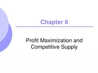
20. Long-Run Market Supply in an Decreasing-Cost Market (b) Market (a) Firm p , $ per unit p , $ per unit 1 MC 2 MC 1 AC 2 AC e E 1 1 p 1 e E 2 2 p 2 S q q q , Units per year Q = n q Q = n q Q , Units per year 1 2 1 1 1 2 2 2

21. downward-sloping LR supply curves: prepared feeds, aircraft, construction equipment, computers, TVs, DVD players, etc. upward-sloping LR supply curves: tires, drugs, paints, glass, etc. flat LR supply curves: plumbing and heating products, floor coverings, etc. on average across all industries: LR supply curves have only slight upward slope LR supply: examples

22. Upward-Sloping Long-Run Supply Curve for Cotton in the world market Price, $ per kg Iran S 1.71 United States 1.56 Nicaragua, Turkey 1.43 Brazil 1.27 Australia 1.15 Argentina 1.08 Pakistan 0.71 0 1 2 3 4 5 6 6.8 Cotton, billion kg per year

23. 9. Applying the competitive model 9.1. Consumer and producer surplus 9.2. Impact of price interventions 9.3. Tax incidence analysis 9.4. Trade restrictions 9.5. Applications

24. 9.1. Consumer and producer surplus (1) Consumer surplus (review) -- Definition (interpretation) -- How to calculate it at a particular price? -- How to calculate the change in consumer surplus due to a tax or a change in price?

25. 9.1. Consumer and producer surplus (2) What is producer surplus? Example: A firm with a supply function qs = -10 + P --------------------------------------------------------------------------- Minimum price to Cumulative P qs supply the last unit “revenue” -------------------------------------------------------------------------- < 10 0 = 11 1 11 11 = 12 2 12 23 = 13 3 13 36 = 14 4 14 50

26. 9.1. Consumer and producer surplus (2) What is producer surplus? Example: A firm with a supply function qs = -10 + P Cumulative “revenue” from 4 units = $50 Total actual revenue from 4 units = 4 x 14 = $56 The difference = 56 - 50 = $6 (producer surplus) Producer surplus: The extra value producers get for a good in excess of the opportunity costs of producing the good.

27. 9.1. Consumer and producer surplus (3) Economic efficiency (Fig. 9.1.) The sum of producer surplus and consumer surplus is at the maximum when the market is at equilibrium. (4) How to estimate consumer & producer surplus? e.g., QD = 10 - P and QS = 0.5 P - 2 At the equilibrium: Q* = 2 and P* = 8 Consumer surplus = 0.5 x 2 x 2 = 2 Producer surplus = 0.5 x 4 x 2 = 4 What will be the change in CS and PS if Q is restricted to be 1.5 units by a quota? If the government wants to reduce Q to 1.5 units by a sales tax, what should be the tax rate per unit?

28. 9.2. Impact of price interventions (1) Price interventions: (2) Impacts of a price ceiling -- If the ceiling price is above the equ. price -- If the ceiling price is below the equ. price Quantity Price Consumer surplus Producer surplus Efficiency -- Examples:

29. 9.2. Impact of price interventions (3) Impacts of a price floor -- If the floor price is below the equilibrium price -- If the floor price is above the equ. price Quantity Price Consumer surplus Producer surplus Efficiency -- Examples