Divide & Conquer Sorting Methods Overview
Explore Merge Sort and Quick Sort algorithms in sorting methods analysis, implementations, and complexities. Understand how divide and conquer techniques optimize sorting efficiency.

Divide & Conquer Sorting Methods Overview
E N D
Presentation Transcript
Sorting Algorithms (Part II) Overview • Divide and Conquer Sorting Methods. • Merge Sort and its Implementation. • Brief Analysis of Merge Sort. • Quick Sort and its Implementation. • Brief Analysis of Quick Sort. • Preview: Searching Algorithms. Sorting Algorithms (Part II)
Divide & Conquer Sorting Methods • In the last lecture, we studied two sorting methods, both of which are quadratic. That is, they are said to be of order n2. • An interesting question to ask is, can we have a linear sorting method – one involving order n comparisons and order n data movements. • The answer to this question is generally no. However, we could have something in-between. • The two methods we are considering in this lecture, namely merge sort and quick sort, are of order n log2n. • Both these methods take an approach called divide and conquer approach, usually implemented using recursion. • In this approach, the array is repeatedly divided into two until the simplest sub-divisions (containing one element) are obtained. These subdivisions which are automatically sorted are then combined together to form larger sorted parts until the entire array is obtained. Sorting Algorithms (Part II)
Merge Sort: An Implementation • This is sometimes called EasySplit/HardJoin as the main work is in the merging part. • Its algorithm consists of the following steps: • 1. Split the list into two equal (or nearly equal) sub-lists – since smaller lists are easier to sort. • 2. Repeat the process on the sub-list (recursively) until all the sub-lists are of order1 – which means they are already sorted. • 3. Rewind the recursion by merging the sub-lists to form larger sorted list. At the end, the original list would have been sorted. • 4. The following diagram illustrates merge sort. Sorting Algorithms (Part II)
Merge Sort: An Implementation (Cont’d) • The following diagram illustrates the merge sort algorithm: Sorting Algorithms (Part II)
Merge Sort: An Implementation (Cont’d) Sorting Algorithms (Part II)
Merge Sort: An Implementation (Cont’d) Sorting Algorithms (Part II)
Brief Analysis of Merge Sort • First we notice that the main work is being done by the merge() method – this is where both the comparison and data movement takes place. • The number of comparisons in the merge() method depends on the number of elements in the sub-list and their ordering. However, since all the elements must be moved to temporary array and moved back to the sub-list, the number of moves is twice the size of the sub-list. • At the top-level for example, at most n key comparison is made and 2n data movements. • As we go down the recursive levels, the size reduce by half each time, but the number of recursive calls increase by the same factor so that the overall number of comparison is n at each level as shown by the following diagram: Sorting Algorithms (Part II)
Brief Analysis of Merge (Cont’d) • The complexity of Merge Sort is “nlog n”. Recurrence relation is used to compute the complexity of merge sort [ics 353 course]. • One disadvantage of merge sort is that a separate array of the same size as the original is required in merging the sub-lists. This takes extra space and computer time. Sorting Algorithms (Part II)
Quick Sort: An Implementation • Quick sort is another divide-and-conquer algorithm that spends more time in the partitioning than merge sort, as such it is sometimes called HardSplit/EasyJoin. • To do the partitioning, Quick Sort first selects an element called the pivot and conceptually divides the list into two sub-lists with respect to the pivot: the first sub-list consisting of all elements less than or equal to the pivot and the second consists of all elements that are greater or equal to the pivot. • These two sub-lists are then sorted using the same idea. By the time the list reduces to single elements, the list would have been sorted. • The partitioning is achieved by using two variables, left and right which are initially set to the first and last index and allow them to move towards each other. • The left variable is allowed to increase until it reaches an element greater to the pivot. • Similarly, the right variable is allowed to decrease until it reaches an element less than the pivot. • Provided the two variables do not cross, the elements they point to are swapped, after swaping left is increase and right is decrease by 1. This process continues until the variables cross each other, at which stage the partition would have been achieved. • The pivot could be any element, but for simplicity we take the middle element. Sorting Algorithms (Part II)
Quick Sort: An Implementation (Cont’d) • The following set of diagrams shows how quick sort works: • Original list: • First we choose a pivot, the middle element = 55. • Left will move and stop at 81, since 81>55; while right cannot move since 23<55 • At this point, the two elements are swapped & variables left++, right-- • Next, left moves and stops at 55, while remain at 17. After swapping and left++ and right-- we get: Sorting Algorithms (Part II)
Quick Sort: An Implementation (Cont’d) • Next, left remain at 65 and right moves and stops at 17. Since the two variables have cross each other, we do not swap, instead we have the following: • Since the variables have crossed, this terminate the first partitioning process, with the two parts as follows: • The process is then repeated with each of the sub partition. Sorting Algorithms (Part II)
Quick Sort: An Implementation (Cont’d) Sorting Algorithms (Part II)
Brief Analysis of Quick Sort • Complexity of Quick Sort is nlog n. • Again, most of the work is done by the partition() method which does. both the comparisons and data movements. • The number of comparison depends on the size of the sub-list being considered and like merge sort, it is at most n for each level of recursion. • However, the number of data movements depends not only on the size of the sub-list, but also on choice of the pivot and the relative ordering of the keys. It is at worst equal to the size of the list (max n) but can be considerably less. • The next question is how many level of recursion are involved? This again depends on the choice of pivot. A good choice of pivot will divide the list into two nearly equal sub-lists. However, in practice, because quick sort performs less number of data movements, it is much faster than merge sort. Sorting Algorithms (Part II)