Download
1 / 36
360 likes | 381 Views
Explore correction methods for MODIS ocean data, including inter-detector balancing, cross-scan corrections, and gain adjustments by the Miami MODIS Science Team. Learn about addressing instrument effects and achieving precise results over time.

E N D
Latest Terra-MODISOcean Color Radiance Corrections Inter-detector, Mirror Side, Cross-Scan, and Gain Adjustments Bob Evans, Ed Kearns, Kay Kilpatrick Rosenstiel School of Marine and Atmospheric Science University of Miami MODIS Science Team Meeting Baltimore, MD. July 2004
Examples of Instrument effects before and after corrections – Figures 1a and b show the effects of mirror side and inter-detector banding. These instrument artifacts are a result of incomplete polarization correction (10 km wide mirror side banding) and detector gain characterization or an as yet unidentified sourceand introduces trends across the focal plane (1km stripes and mirror side trends). Mirror side difference, Figure 1a, is AOI and time dependent, order ±1.5% Lt; Figure 1b shows the average detector-to-detector trends in gain that are necessary to minimize cross-focal plane trends and detector stripes, order ±0.2% Lt.
Typical Problems • Single-pixel high stripes in 1km data • Interdetector mismatches in bands • 10-pixel high stripes • Mirror-side differences • Bias and RVS • Edge-to-Edge of Swath discontinuities • Unresolved RVS variations • Temporal inconsistencies in nLw • LUT’s m1 values not precise enough • Low-level changes
Basic Methodology • Use Terra-MODIS time series at Hawaii • >1200 days/granules • MOBY time series • Break time series into “epochs” • Accounts for instrument changes not well resolved in m1’s
Interdetector balancing: remove “single-pixel” striping • Correct on a per band, per epoch basis • Use a modal analysis to determine peak response of each detector • Requires multiple granules per epoch for adequate resolution • Adjust modal peak for each detector to match that for detector 5 • Relatively easy to achieve • Same technique can be done with x-scan dependence if need be….new polarization table has reduced the need somewhat
Cross Scan corrections • Requires “flat field” assumption: no significant, consistent zonal gradients near Hawaii • Compute average cross-scan distribution per granule for each band, relative to the position at pixel 500 (west of nadir for Terra Day) • Group the granules’ x-scan behavior within each epoch • Avoid sun glint contamination!! • Fit a 5th order polynomial in a least-squares sense to normalize the distribution • Quantize this correction into 50 x-scan correction values. High AOI shows the most change. xscan carries bulk of the correction.
Shape of x-scan correctionfor each epoch 412nm Low AOI High AOI
Balance Mirror Side 2 • Add detector bias and cross-scan correction to 2nd mirror side to match first mirror side • Does not require a significant flat-field assumption, but assumes that the optical meridional variability in the ocean near Hawaii on the scale of 10km is small • Compute average mirror side difference for each granule as a function of x-scan position • Fit a 5th order polynomial to the mirror side differences for all granules within an epoch • Quantize this as a 50 element correction vector
Net correction applied to Mirror 2 443nm east East high aoi West low aoi nadir
Net correction applied to Mirror 2 412nm west low AOI East high AOI nadir
Example: Day 2004 1131km L2 magnified • nLw 412nm • Hardest to do • Note relatively good corrections right up to sun glint • Works well over wide range of Lt’s
Day 22, Year 2004 nLw 412nm Note mirror-side striping only in upper right
Setting the final gainsnLw to Lt to nLw to Lt… • Radiance deficits and anomalies are detected and measured in nLw space (L2) • Corrections are applied to Lt values (L1B) • Requires a recursive method • Estimate nLw radiance error • Scale to Lt • Per band • Systematically underestimate to account for variability • Repeat until solution converges
Gain correction • Implement an overall exponential correction for blue Bands 8 and 9 (based on mean MOBY behavior), not per epoch • Adjust Bands 10, 11, 12 on a per epoch basis • Adjust MODIS (Band X / Band 9) to match MOBY (Band X / Band 9) ratio • Want ratios (products) to be stable • Aim for low RMS • Neglect MOBY v. MODIS individual band bias • Adjust 748nm band (linear/exponential) to remove long-term trends in mean epsilon fields
Modal time series • Use a time series of the mode of each MODIS band’s data in a small concentric circles (30, 10, and 3 km) around MOBBY with increasing weights • Compare to filtered MOBY data time series
Time series 443 • Modal time series • % difference from MOBY (red points matchup pairs, blue bar epoch average) • ratio mode/measured
Time series 551nm • Modal time series 551nm • % difference from MOBY (red points matchup pairs, blue bar epoch average) • Time series blue/green ratio
Net gains in time • Gains are computed per band for each epoch • Multiply the gain by the xscan correction for west, center, and east side of scan for each epoch
443nm net correctiongain * xscan for each epoch west low AOI East high AOI nadir
Top panel - radcor gain vs time, purple line is band 8 gain adjustmentBottom panel - deviations of the measured m1 coefficients from the linear trends band 8, mirror side 0 (corrected) [from Gerhard Meister]Radcor oscillations ~ factor 5 large than SD M1 trend residualsNote: Radcor time resolution ~60 days, M1 two weeks
551nm net correctiongain * xscan for each epoch west low AOI East high AOI nadir
Gain corrections for MODIS-TerraRed - 667, 678nm, Green - 551nm, Yellow - 531nm, Blue - 443nm, Purple - 412nm TERRA 041 reprocessing gains Calibration adjustments developed for current MODIS ocean reprocessing Blue bands fit to winter MOBY nLw observations to minimize sun-glint and polarization issues. Green bands adjusted to match MODIS to MOBY blue/green band ratios. Days since Jan 1, 2000 to Dec 31, 2003
Smoothing net corrections exponential least square regression551nm Example: Nadir xscan
Improvements in terra_v24_49 • Smoother gain evolutions • No seasonal oscillations • No need for additional smoothing • More predictable x-scan and mirror side • Overall we have been able to remove much of the problems in the l1b data that were present in the transition between 2003 and 2004.
Bias and RMS terra_v24_49 N = 15
Remaining Problems • Remaining sun glint contamination (x-scan)? • Still some odd behavior, variable in time & space • No other guidance for red bands (fluorescence) • Requires set balancing of 667/678nm ratio • Some per-detector xscan behavior remains (though less than before). The time trend in the cross scan correction at high AOI likely indicates a change in the mirror polarization. • Still data and time intensive • Terra_v24_50 still has a few issues to be fixed • Red gains still maladjusted for 2 or 3 epochs • Inter-detector balance off for 2 epochs for Band 12
Smoothing and prediction (experimental) • Fit bicubic splines under tension to net cross-scan behavior • Caveats: avoid summer times (residual glint)? Edge of scan? • Produces look-up tables and functional relationships for corrections • Limited predictive capabilities (good enough for short term?)
xscan pixel Day of year 2000
xscan pixel Day of year 2000