Download
1 / 48
480 likes | 589 Views
PhD Course: Performance & Reliability Analysis of IP-based Communication Networks. Henrik Schiøler, Hans-Peter Schwefel, Mark Crovella, Søren Asmussen. Day 1 Basics & Simple Queueing Models(HPS) Day 2 Traffic Measurements and Traffic Models (MC)

E N D
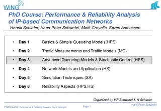
PhD Course: Performance & Reliability Analysis of IP-based Communication Networks Henrik Schiøler, Hans-Peter Schwefel, Mark Crovella, Søren Asmussen • Day 1 Basics & Simple Queueing Models(HPS) • Day 2 Traffic Measurements and Traffic Models (MC) • Day 3 Advanced Queueing Models & Stochastic Control (HPS) • Day 4 Network Models and Application (HS) • Day 5 Simulation Techniques (SA) • Day 6 Reliability Aspects (HPS,HS) Organized by HP Schwefel & H Schiøler
Reminder: Day 1 – Exponential models • Intro & Review of basic stochastic concepts • Random Variables, Exp. Distributions, Stochastic Processes • Markov Processes: Discrete Time, Continuous Time, Chapman-Kolmogorov Eqs., steady-state solutions • Simple Qeueing Models • Kendall Notation • M/M/1 Queues, Birth-Death processes • Multiple servers, load-dependence, service disciplines • Transient analysis • Priority queues • Simple analytic models for bursty traffic • Bulk-arrival queues • Markov modulated Poisson Processes (MMPPs) • MMPP/M/1 Queues and Quasi-Birth Death Processes
Reminder: Day 2 – Traffic Properties • Properties of Network Traffic • Daily/weekly profiles • Burstiness/Long-Range Dependence/Self-Similarity • Application specific properties • Impact of Transport Protocols (in particular TCP) • Actual Measurements(ATM-basedGerman University backbone, 1998)inter-cell times Xi: • C2(X) between 13,…,30 • positive autocorrelation coefficient:ř(k) = (i(Xi-x)(Xi+k-x)) / Var(X) > 0, slowly decaying with k Correlation Plot (Inter-cell times)
Content • Matrix Exponential (ME) Distributions • Definition & Properties: Moments, distribution function • Examples • Truncated Power-Tail Distributions • Queueing Systems with ME Distributions • M/ME/1//N and M/ME/1 Queue • ME/M/1 Queue • Performance Impact of Long-Range-Dependent Traffic • N-Burst model, steady-state performance analysis • Transient Analysis • Parameters, First Passage Time Analysis (M/ME/1) • Stochastic Control: Markov Decision Processes • Definition • Solution Approaches • Example Note: this slide-set contains only the outline of the lecture; many formulas and the mathematical derivations will be presented on the black-board!
Notation (Summary) • Matrices: underlined capitals: B , V, ... • Unit Matrix: I= diag([1,1,…,1]) • Row vectors: underlined, lower-case: p, u, … • Column vectors: primed • ’ = [1,1,…,1]’ • Random Variables: Capitals: X, U, … • Expected Values: E{X}, E{X2},… • Coefficient of correlation: r(X,Y)=E{(X-E{X})*(Y-E{Y})} / (std(X)*std(Y))auto-correlation coefficient (process (Xi) ): r(k) = r(Xi, Xi+k) • Queueing Systems: • Infinite buffer: G/G/1 • Finite loss systems: G/G/1/B • Finite number of customers: G/G/1//K
Matrix Exponential Distributions • Replace single state with open system S containing m states, described by • Entrance vector p=[p1,…, pm] • State leaving Rates: M=diag(1,…,m) • Transition Probabilities: P=(pij) • Note: q:= ’ - P’ 0 (in contrast to discrete time Markov chains) • Interested in Random VariableX:= time to leave S | entered according to p
Matrix Exponential Distributions: Properties • Mean Time to leave S:where • Trivial Example: Exponential distribution, E{X}=pV’=1/ • Distribution of X: • Density: f(x)=- dR(x)/dx = pB exp(-xB) ’ • k-th Moments: • Matrix Exponential Distributions Phase-Type Distributions
Examples I: Hyper-exponential Distributions • Weighted Mixture of two (or m) exponentials: • Moments: frequently used to approximate distributions with high variance • Matrix-Exponential Representation: <p,B>
Examples II: Erlangian Distributions • Sum of T exponentially distributed RVs • Probability density function: • Moments: • Limit (T, T~1/T): deterministic RV • Matrix-Exponential Representation
Examples III: (Truncated) Power-Tail Distributions • Definitions: • Sub-exponential distributions • Power-Tail distributions • Example: Pareto Distribution • Properties: • Moments • Residual Times • Truncated Power-Tail Distributions • Representation as hyper-exponentials • Systematic control of Power-tail Range • [easy to generate in simulation models]
Content • Matrix Exponential (ME) Distributions • Definition & Properties: Moments, distribution function • Examples • Truncated Power-Tail Distributions • Queueing Systems with ME Distributions • M/ME/1//N and M/ME/1 Queue • ME/M/1 Queue • Performance Impact of Long-Range-Dependent Traffic • N-Burst model, steady-state performance analysis • Transient Analysis • Parameters, First Passage Time Analysis (M/ME/1) • Stochastic Control: Markov Decision Processes • Definition • Solution Approaches • Example
M/G/1 and M/ME/1 Queueing Models • Poisson Arrivals (rate ) • service times general (ME) distributed (i.i.d. RVs Xi, described by <p,B>) • Utilization: = E{X} [ Pr(Q=0)=1- for infinite buffer model, as we will see later] • Solution Approaches: • Embedded Markov Chain (see e.g. Kleinrock)Pollaczek-Khinchin Formula: • Quasi-Birth Death Processes existence of Matrix-geometric solution • Limit of finite-customer systems: M/ME/1//N models
M/ME/1//N Queueing Systems: steady state queue-length distribution • Define • r(n;N) := Pr(’n customers at S1’) • ((n;N))i := Pr(’n customers at S1 & server S1 in state i’) • Balance Equationswith • Matrix-Geometric Solution
M/ME/1//N Queueing Systems (cntd.) • Normalization (r(n)=1) • Probabilities at • Arrival instances • Departure instances
ME/M/1 Queueing Systems • Definition: • Service Times exponential (rate ), • Inter-Arrival Times Xi iid, described by <p,B>) • In principle same approach as for M/ME/1: • Existence of Matrix-geometric solution known from QBD theory • Consider solution of finite ME/M/1//N system • Take limit N • Finite ME/M/1//N system identical to M/ME/1//N system (but consider S2 instead of S1) • = 1 / [E{X}] • Obstacles • Lim UN does not exist (U has eigenvalues > 1) consider lim sNUNwhere s is the smallest eigenvalue of A
ME/M/1 Queueing Systems: Solution • Solution (Matrix-geometric solution reduces to geometric!) • Performance Parameters
Exercise 1: • ME distributions • M/ME/1 Queue • ME/M/1 Queue Detailed tasks, see attached sheet.
Content • Matrix Exponential (ME) Distributions • Definition & Properties: Moments, distribution function • Examples • Truncated Power-Tail Distributions • Queueing Systems with ME Distributions • M/ME/1//N and M/ME/1 Queue • ME/M/1 Queue • Performance Impact of Long-Range-Dependent Traffic • N-Burst model, steady-state performance analysis • Transient Analysis • Parameters, First Passage Time Analysis (M/ME/1) • Stochastic Control: Markov Decision Processes • Definition • Solution Approaches • Example
Reminder: Self-Similarity/Long-Range Dependence • Self-Similarity with Hurst Parameter H: [Ni()]i = [s-H Nj(s)]j d • Second Order Self-Similarity: r(m)(k) r(k) for all m,k=1,2,.... • where r(m)(k) is autocorrelation of averaged, m-aggregated process • Asymptotic Second Order Self-Similarity: lim r(m)(k) / r(k) = 1 • for all m=1,2,... k • Long-Range Dependence: r(k) (assuming r(k)0 ) • with special case:r(k) ~ 1/k(-1) , 1<<2 • The latter processes are asymptotically second order self-similar!
Self-Similar/LRD Traffic Models • Fractional Brownian Motion / Fractional Gaussian Noise N(t) = m t + sqrt(a m) Z(t) where Z(t) continuous, normally distributed, E{Z2}= t2H , 0.5<H<1 ... is self-similar with parameter H and long-range dependent with =3-2H • ON/OFF Traffic with Power-Tailed ON periods (1< <2)... is long-range dependent • ... [others, e.g. chaotic maps, F-ARIMA]
ON/OFF Models • Parameters: • N sources, each average rate • During ON periods: peak-rate p • MMPP representation(exponential case): • Mean duration of ON and OFF times • ON times general Matrix exponential:<p,B>: Pr(ON>t) = p exp(-Bt)´ N
MMPP Representation: Multiplexed ON/OFF models i=1 (needed for TCP models, not done here)
N-Burst with TPT-T ON-time distribution • Power-Tail distribution Very long ON periods can occur • Exponent : Heavier Tails for lower ; Impact on exponent in AKF • Truncated Tail: Power-Tail Range, Maximum Burst Size (MBS)
N-Burst /M/1 Performance: Blow-up Points • Power-Tailed queuelength-distr. • ...with changing exponents (i0) • Tail truncated at qN(MBS) • `Blow-up Regions´ i0=1,...,N for LRD traffic • Radical delay increase at transitions
Cause of Blow-up Regions • Oversaturation periods caused by a mimimum of i0 long-term active sources • Duration of oversaturation periods: PT with exponent =i0(-1)+1 matters for performance, not or H
Consequences: Power-Laws for BOP & CLP • Buffer Inefficiency: BOP ~ B1-CLP ~ B1- • Drop-off for B>qN • Power-Law growth of mCD(MBS) when <2 BUT: Steady-State reached in 4-8 daily Busy Hours ? BOP = Buffer Overflow Probability (N-Burst/M/1) , CLP = Cell Loss Probability (N-Burst/M/1/B)
Looking at Burstiness once more • Def. (see Day1): range b=0 (not bursty) to b=1 (very bursty): b:=1-/p , Average Rate of Source , Peak Rate of Source p • Investigating burstiness: • Vary p • Keep #packets per ON period scale ON duration accordingly • Extreme Cases: • b=0 (p=): Poisson arrivals, no burstiness • b=1 (p=): Bulk arrivals • Mean packet delay shown for • Single ON/OFF source (N=1) • Utilization =0.5 • Tail Exponent =1.4 for ON periods
Fluid-Flow or Point-Process Models? • Experiment: scale ’packet-size’ by factor k • Packet rate p k p , service rate k • Limit: • k: fluid-flow model • Mean packet delay shown for • Single ON/OFF source (N=1) • Utilization =0.5 • TPT-30 distribution withTail Exponent =1.4 for ON periods
Content • Matrix Exponential (ME) Distributions • Definition & Properties: Moments, distribution function • Examples • Truncated Power-Tail Distributions • Queueing Systems with ME Distributions • M/ME/1//N and M/ME/1 Queue • ME/M/1 Queue • Performance Impact of Long-Range-Dependent Traffic • N-Burst model, steady-state performance analysis • Transient Analysis • Parameters, First Passage Time Analysis (M/ME/1) • Stochastic Control: Markov Decision Processes • Definition • Solution Approaches • Example
Transient Behavior: Motivation Simulation: Fraction of overflowed packets • Example: • ON/OFF traffic with TPT ON time • Queueing Model with large buffer • Observations (Simulation): • Highly correlated overflow events • Large fluctuations between different observation intervals • Steady-state Overflow-Prob.not always meaningful Transient analysis necessary
Transient Analysis: Basics • Selected transient parameters • Transient Queue-length Probabilities: Pr(Q(t)=n) • First Passage Time AnalysisFPT(n) = RV reflecting the time until the buffer occupancy reaches level n for the first time (given some well-defined initial state, normally empty queue) • Busy Period Analysis • Duration of busy period • Pr(buffer occupancy reaches maximum QL n during busy period) • Transient Overflow Probabilities:(t,n) = Pr(FPT(n)<t) • Transient parameters depend on initial conditions • E.g. Empty queue (Q(0)=0), state of arrival process, state of service process (for correlated service events)
Computation of mean First Passage Times: demonstrated for M/ME/1 Queues • Poisson Arrivals (rate ), service times <p,B> • Approach: • [pu(i)]j:=Pr(server in state j when queue reaches level i for the first time) • [u(i)]j:= Mean time it takes to have i+1 customers for the first time, given started at queue-length i in server state j • Introduce Matrix • [Hu(n)]ij:=Pr(server in state j when queue goes from level nn+1 for the first time , given server started in state i at queue-length n) • Rewrite
Computation of mean First Passage Times: recursive equations • Recursive Equations for Hu(n) • Similarly for u(i)
Example:Mean First Passage Times N-Burst/M/1 • mFPT grows by Power-Law B similar blow-up effects for changing as for steady-state analysis
Optional: Traffic/Performance Models for TCP End-to-End flow/congestion control Feedback: network behavior (congestion) ingress traffic • No separation traffic model/network model possible • New traffic/performance models required Approaches: • Connection level models • Sender/receiver behavior & fixpoint iteration • Integrated models Traffic Model Network Model Performance Values(Delay, Loss, etc.) feedback
Example: Fixpoint Iteration Update: loss rate p, delay d Initial loss rate p, delay d TCPModel Network Model When stable: result Average packet rate • Network Model: • E.g. M/M/1/K model or bulk-arrival queue • TCP model, e.g. [Padhye et al., Sigcomm 98] • b: # packets acknowledged by ACK • RTT: Average Round-Trip-Time (including queuing delay) • Wmax: Maximum size of congestion window • T0: Average Time-Out interval • p: Fraction of retransmitted packets
HTTP TCP IP Link-Layer L5-7 L4 L3 L2 Traffic Modelling Challenges • Multiplexing of packets at nodes (L3) • Burstiness of IP traffic (L3-7) • Impact of Routing (L3) • Performance impact of transport layer, in particular TCP (L4) • Wide range of applications different traffic & QoS requirements (L5-7) Day1 & 3 [touched] Traffic Model Network Model Performance Values(Delay, Loss, etc.) TCP / adaptive applics. Wireless Link Properties Mobility Model
Content • Matrix Exponential (ME) Distributions • Definition & Properties: Moments, distribution function • Examples • Truncated Power-Tail Distributions • Queueing Systems with ME Distributions • M/ME/1//N and M/ME/1 Queue • ME/M/1 Queue • Performance Impact of Long-Range-Dependent Traffic • N-Burst model, steady-state performance analysis • Transient Analysis • Parameters, First Passage Time Analysis (M/ME/1) • Stochastic Control: Markov Decision Processes • Definition • Solution Approaches • Example
Markov Decision Processes: Motivation & Definition • Markov Process definition • State-Space • Transition Probabilities/Rates • Computation of System behavior (e.g. performance parameters) Extension: Investigate ’optimal control’ of such a Markov model • Markov Decision Processes (MDPs) • State-Space E • Actions: a(s,t) A, sE • Transition Probabilities depend on current state s(t) and on selected action a(s,t) • Rewards [Costs/Utility]: r(s,a) • Goal: Find ‘selection of actions’ that maximize some reward criterion • Simple Example: extended Gilbert-Elliot Channel Model
MDPs: Policies • Policies • =(d1,d2,...), sequence of decision rules • Decision rules: di: EA -- specification of action depending on state s • Types of Policies • Randomized vs. deterministic • Stationary vs. non-stationary • For a given stationary, deterministic policy=(d,d,...), the MDP is a (homogeneous) Markov process, enriched by the reward function, r(s,d(s))
MDPs: Optimality Criterions [Assumptions: discrete time, finite action space] Optimality criterion: Maximize expected reward • Finite horizon (covering N steps) vN, (s0)=E,s0{ r(Xi, d(Xi) }[sum runs from i=1 to N] • Infinite horizon • Total expected reward v (s0)=E,s0{ r(Xi, d(Xi) }[sum runs from i=1 to ] • Expected average reward v (s0)=lim 1/N E,s0{ r(Xi, d(Xi) }[sum runs from i=1 to N; lim N] • Total expected discounted reward v (s0)=E,s0{ i r(Xi, d(Xi) }[sum runs from i=1 to ] , 0<<1 • for stationary policy =(d,d,...) and initial state X0=s0
MDPs: Solution Approaches and applications ’Learning’ Approaches: • Neural Networks • Genetic Algorithms • Q-Learning Solution Approaches: • Value iteration • Policy iteration • Linear Programming • Dynamic Programming Applications: • Call admission control & handoff control • Paging/mobility tracking • Radio Resource Management • Scheduling/Buffer Management • Routing
MDPs: References • Cassandras, Lafortune, ’Introduction to Discrete Event Systems’, Chapt. 9, 1999. • Heyman, Sobel (ed.), ‘Stochastic Models’, Chapt. 8, 1990 • Bertsekas, ‘Dynamic Programming and Stochastic Control’, 1976 • Martin.L.Puterman, Markov Decision Processes: Discrete Stochastic Dynamic Programming, John Wiley & Sons, Inc. 1994. • R.Ramjee, R.Nagarajan and D.Towsley, On Optimal Call Admission Control in Cellular Networks, IEEE INFOCOM 1994 • R.Rezaiifar, A.Makowski and S.Kumar, Stochastic control of Handoffs in Cellular Networks, IEEE JSAC, vol.13., no.7. 1995 • El. El-Alfi, Y.Yao, H.Heffes, A Model-Based Q-Learning Scheme for Wireless Channel Allocation with Prioritized Handoff, IEEE Globecom 2001. • U.Madhow, M.L.Honig, and K.Steiglitz, Optimization of Wireless Resources for Personal Communications Mobility Tracking, IEEE INFOCOM, 1994. • V.Wong, V.Leung, An Adaptive Distance-Based Location Update Algorithm for Next-Generation PCS Networks, IEEE JSAC,vol.19,no.10,Oct.2001. [Acknowledgment:List of References partially from Presentation of Bang Wang, NUS, Sept. 02]
Summary • Matrix Exponential (ME) Distributions • Definition & Properties: Moments, distribution function • Examples • Truncated Power-Tail Distributions • Queueing Systems with ME Distributions • M/ME/1//N and M/ME/1 Queue • ME/M/1 Queue • Performance Impact of Long-Range-Dependent Traffic • N-Burst model, steady-state performance analysis • Transient Analysis • Parameters, First Passage Time Analysis (M/ME/1) • Stochastic Control: Markov Decision Processes • Definition • Solution Approaches • Example
Exercises II: Complete Exercise 1d (transient analysis)