Chapter 52
Chapter 52. Population Ecology. Overview: Earth’s Fluctuating Populations To understand human population growth We must consider the general principles of population ecology. Population ecology is the study of populations in relation to environment

Chapter 52
E N D
Presentation Transcript
Chapter 52 Population Ecology
Overview: Earth’s Fluctuating Populations • To understand human population growth • We must consider the general principles of population ecology
Population ecology is the study of populations in relation to environment • Including environmental influences on population density and distribution, age structure, and variations in population size
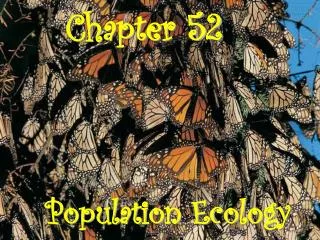
The fur seal population of St. Paul Island, off the coast of Alaska • Is one that has experienced dramatic fluctuations in size Figure 52.1
Concept 52.1: Dynamic biological processes influence population density, dispersion, and demography • A population • Is a group of individuals of a single species living in the same general area
Density and Dispersion • Density • Is the number of individuals per unit area or volume • Dispersion • Is the pattern of spacing among individuals within the boundaries of the population
Density: A Dynamic Perspective • Determining the density of natural populations • Is possible, but difficult to accomplish • In most cases • It is impractical or impossible to count all individuals in a population
Births and immigration add individuals to a population. Births Immigration PopuIationsize Emigration Deaths Deaths and emigration remove individuals from a population. • Density is the result of a dynamic interplay • Between processes that add individuals to a population and those that remove individuals from it Figure 52.2
Patterns of Dispersion • Environmental and social factors • Influence the spacing of individuals in a population
(a) Clumped. For many animals, such as these wolves, living in groups increases the effectiveness of hunting, spreads the work of protecting and caring for young, and helps exclude other individuals from their territory. Figure 52.3a • A clumped dispersion • Is one in which individuals aggregate in patches • May be influenced by resource availability and behavior
(b) Uniform. Birds nesting on small islands, such as these king penguins on South Georgia Island in the South Atlantic Ocean, often exhibit uniform spacing, maintained by aggressive interactions between neighbors. Figure 52.3b • A uniform dispersion • Is one in which individuals are evenly distributed • May be influenced by social interactions such as territoriality
A random dispersion • Is one in which the position of each individual is independent of other individuals (c) Random. Dandelions grow from windblown seeds that land at random and later germinate. Figure 52.3c
Demography • Demography is the study of the vital statistics of a population • And how they change over time • Death rates and birth rates • Are of particular interest to demographers
Life Tables • A life table • Is an age-specific summary of the survival pattern of a population • Is best constructed by following the fate of a cohort
The life table of Belding’s ground squirrels • Reveals many things about this population Table 52.1
Survivorship Curves • A survivorship curve • Is a graphic way of representing the data in a life table
1000 100 Number of survivors (log scale) Females 10 Males 1 2 8 10 4 6 0 Age (years) Figure 52.4 • The survivorship curve for Belding’s ground squirrels • Shows that the death rate is relatively constant
1,000 I 100 II Number of survivors (log scale) 10 III 1 100 50 0 Percentage of maximum life span • Survivorship curves can be classified into three general types • Type I, Type II, and Type III Figure 52.5
Reproductive Rates • A reproductive table, or fertility schedule • Is an age-specific summary of the reproductive rates in a population
Table 52.2 • A reproductive table • Describes the reproductive patterns of a population
Concept 52.2: Life history traits are products of natural selection • Life history traits are evolutionary outcomes • Reflected in the development, physiology, and behavior of an organism
Life History Diversity • Life histories are very diverse
Figure 52.6 • Species that exhibit semelparity, or “big-bang” reproduction • Reproduce a single time and die
Species that exhibit iteroparity, or repeated reproduction • Produce offspring repeatedly over time
Researchers in the Netherlands studied the effects of parental caregiving in European kestrels over 5 years. The researchers transferred chicks among nests to produce reduced broods (three or four chicks), normal broods (five or six), and enlarged broods (seven or eight). They then measured the percentage of male and female parent birds that survived the following winter. (Both males and females provide care for chicks.) EXPERIMENT 100 Male Female 80 60 Parents surviving the following winter (%) 40 20 The lower survival rates of kestrels with larger broods indicate that caring for more offspring negatively affects survival of the parents. CONCLUSION 0 Reduced brood size Normal brood size Enlarged brood size “Trade-offs” and Life Histories • Organisms have finite resources • Which may lead to trade-offs between survival and reproduction RESULTS Figure 52.7
(a) Most weedy plants, such as this dandelion, grow quickly and produce a large number of seeds, ensuring that at least somewill grow into plants and eventually produce seeds themselves. Figure 52.8a • Some plants produce a large number of small seeds • Ensuring that at least some of them will grow and eventually reproduce
(b) Some plants, such as this coconut palm, produce a moderate number of very large seeds. The large endosperm provides nutrients for the embryo, an adaptation that helps ensure the success of a relatively large fraction of offspring. Figure 52.8b • Other types of plants produce a moderate number of large seeds • That provide a large store of energy that will help seedlings become established
Parental care of smaller broods • May also facilitate survival of offspring
Concept 52.3: The exponential model describes population growth in an idealized, unlimited environment • It is useful to study population growth in an idealized situation • In order to understand the capacity of species for increase and the conditions that may facilitate this type of growth
Per Capita Rate of Increase • If immigration and emigration are ignored • A population’s growth rate (per capita increase) equals birth rate minus death rate
dN rN dt • Zero population growth • Occurs when the birth rate equals the death rate • The population growth equation can be expressed as
Exponential Growth • Exponential population growth • Is population increase under idealized conditions • Under these conditions • The rate of reproduction is at its maximum, called the intrinsic rate of increase
dN rmaxN dt • The equation of exponential population growth is
2,000 dN 1.0N dt 1,500 dN 0.5N dt Population size (N) 1,000 500 0 0 10 15 5 Number of generations Figure 52.9 • Exponential population growth • Results in a J-shaped curve
8,000 6,000 Elephant population 4,000 2,000 0 1900 1920 1940 1960 1980 Year Figure 52.10 • The J-shaped curve of exponential growth • Is characteristic of some populations that are rebounding
Concept 52.4: The logistic growth model includes the concept of carrying capacity • Exponential growth • Cannot be sustained for long in any population • A more realistic population model • Limits growth by incorporating carrying capacity
Carrying capacity (K) • Is the maximum population size the environment can support
The Logistic Growth Model • In the logistic population growth model • The per capita rate of increase declines as carrying capacity is reached
Maximum Per capita rate of increase (r) Positive N K 0 Negative Population size (N) Figure 52.11 • We construct the logistic model by starting with the exponential model • And adding an expression that reduces the per capita rate of increase as N increases
(K N) dN rmax N dt K • The logistic growth equation • Includes K, the carrying capacity
Table 52.3 • A hypothetical example of logistic growth
2,000 dN 1.0N Exponential growth dt 1,500 K 1,500 Logistic growth Population size (N) 1,000 dN 1,500 N 1.0N dt 1,500 500 0 0 5 10 15 Number of generations • The logistic model of population growth • Produces a sigmoid (S-shaped) curve Figure 52.12
1,000 800 600 Number of Paramecium/ml 400 200 0 0 5 15 10 Time (days) (a) A Paramecium population in the lab. The growth of Paramecium aurelia in small cultures (black dots) closely approximates logistic growth (red curve) if the experimenter maintains a constant environment. Figure 52.13a The Logistic Model and Real Populations • The growth of laboratory populations of paramecia • Fits an S-shaped curve
180 150 120 90 Number of Daphnia/50 ml 60 30 0 160 0 40 60 100 120 140 20 80 Time (days) (b) A Daphnia population in the lab. The growth of a population of Daphnia in a small laboratory culture (black dots) does not correspond well to the logistic model (red curve). This population overshoots the carrying capacity of its artificial environment and then settles down to an approximately stable population size. Figure 52.13b • Some populations overshoot K • Before settling down to a relatively stable density
80 60 40 Number offemales 20 0 1995 2000 1980 1985 1990 1975 Time (years) (c) A song sparrowpopulation in its natural habitat. The population of female song sparrows nesting on Mandarte Island, British Columbia, is periodically reduced by severe winter weather, and population growth is not well described by the logistic model. Figure 52.13c • Some populations • Fluctuate greatly around K
The logistic model fits few real populations • But is useful for estimating possible growth
The Logistic Model and Life Histories • Life history traits favored by natural selection • May vary with population density and environmental conditions
K-selection, or density-dependent selection • Selects for life history traits that are sensitive to population density • r-selection, or density-independent selection • Selects for life history traits that maximize reproduction
The concepts of K-selection and r-selection • Are somewhat controversial and have been criticized by ecologists as oversimplifications
Concept 52.5: Populations are regulated by a complex interaction of biotic and abiotic influences • There are two general questions we can ask • About regulation of population growth