Theory off chaotic light and coherence

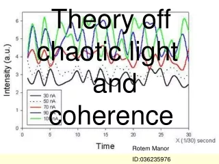
1. Theory off chaotic light and coherence Rotem Manor ID:036235976

2. It is important to distinguish between tow types of light source: • Chaotic source: gas discharge lamp, where the different atoms are excited by an electrical discharge and emit their radiation independently of one another. emission line determined by statistical spread in atomic velocities andrandom occurrence of collisions. • Laser: high intensity ,coherence

3. There are three mechanisms witch are mainly responsible for the spread in frequency of emitted light. The decay process it self:leads to broadening of an absorption line of Lorentzian frequency distribution (with a width Γ). Collision broadening: form the atomic motion. Spread in atomic velocities: leads to Doppler spread in emitted frequencies. Note: it is convenient to neglect the other linewidth contributions while treating a particular broadening process.

4. Doppler broadening Atom in exited energy level , Has velocity . Emits photon of energy and falls to a lower energy level . The photon has a momentum where and is emission causes a recoil of the atom to a new velocity Momentum : Energy: Let be the frequency of light which would be emitted if the atom had zero velocity before and after the emission.

5. It gives us: We’ll take k to be on the z-axis Typical orders of magnitude: Hence There for the frequency of emitted light suffers a Doppler shift.

6. The Maxellian velocity distribution define the frequency distribution where Probability function: where

7. Collision broadening We focus attention on the same pair of atomic states that we have used before, but we now ignore the other linewidth( assumption: the radiative lifetime of an atom is long compared to time between collisions). Consider a particular exited atom radiating light of frequency. When it suffers a collision his energy levels are shifted by the force of interaction between the two colliding atoms. After the collision the wave frequency is resumed with all the other characteristics, except from the phase of the wave, that is unrelated to the one before the collision. If the duration of the collision is sufficiently brief, it is possible to ignore any radiation emitted during the collision while is shifted. The collision broadening effect can then be adequately represented by a model in witch each exited atom always radiates at frequency , but with random changes in the phase of radiated wave each time a collision occurs.

8. The wave train radiated by single atom. Vertical line represent a collision. The Phase of The wave train radiation According to the kinetic theory of gases, the probability that an atom has period of free flight lasting a length of time between t and t+dt is Hence

9. If we consider one period of free flight of an atom, The field can be written in a complex form: And represent as a Fourier integral

10. Thus the cycle averaged intensity is

11. At any instant of time the total intensity of radiation is made up of contribution from large number of exited atoms. The probability of the free flight time is given( in slide 8 ), so it’s necessary to integrate the intensity with the probability over time for getting the total intensity. realistic values for gas in room temperature and pressure . So average atom doing about 15,000 periods of oscillations before a collision, And the collision linewidth is about 100 times the natural radiative linewidth( Г )

12. Composite emission lineshape It is interesting to note that the Doppler width( slide 6 ) is approximately equal to the collision linewidth for this parameter values. In this case it is necessary to determine the composite lineshape of all the dominant processes. A combination of two line broadening mechanisms with individually generate normalized lineshape functions f(ω) and g(ω) is Where is the common central frequency component of the distributions. Clearly if the two sources of broadening are Lorentzians And for Gaussians

13. Time dependence of the chaotic light beam It is clear from the above discussions that the frequency spread of the emitted light is governed by the same physical parameters as the time dependence of emitting source atom. The wave train emitted by a single atom( number 1 ) is The total emitted wave is represented by a sum of this terms For simplicity we will assume that the observed light has a fixed polarization so that the electric field can be added algebraically

14. The amplitude a(t) is illustrated in this diagram and are different and different instate of time.

15. How ever it is not possible in practice to resolve the oscillation in E(t) witch occur at the frequency of the carrier wave. A good experimental resolving time is of the order (six order magnitude too long to detect the oscillation of the carrier wave). The real electric field has zero cycle average and the beam intensity in free space is

16. This is a computer simulation of a collision-broadened light source. • It is seen that substantial changes in intensity and phase can occur over time span , but these quantities are reasonably constant over time intervals • . • It gives us two new parameters • - coherence time, • - coherence length.

17. Intensity fluctuation of chaotic light Intensity fluctuation can be measured experimentally only with a detector whose response time is short compared to the coherence time . So a normal detector is measuring averages. (the bar denotes a long tome average for a time long compared to ) So the long time average intensity is It is seen that in any instant of time the movement of a(t) is in depend on steps in random direction like in the ‘random walk’ problem, so let p[a(t)] be the probability of the end point of a(t).

18. Probability distribution for the amplitude and the phase of electric field of chaotic light

19. If we’ll calculate: It’s means that the fluctuation are . Despite the very large fluctuation compared to the intensity, the coherence time is usually so short that it is difficult to observe the fluctuation in experimentally and their influence is often small.

20. Young’s interface fringes The model experiment ignores complications arising from the finite source diameter and consequent lack of parallelism in the beam witch illuminates the first screen.

21. Let E(r,t) be total electric field of radiation at position r on the observation screen at time t. Where And are inversely proportional to respectively, and depend on the geometry of the experiment. The intensity of the light in the position r averaged on over a cycle of oscillation is

22. The fringes in Young’s interface experiment are normally can be observed by the naked eye. In this case the recording time is long compared to and there for it is necessary to average . Where The first two terms represents the intensities caused by each pinholes in the absence of others. The third one is called first-order correlation function of the field, and it’s clearly depend on (the deference between the times at witch the fields are measured).

23. Evaluation of the first order correlation function Let’s calculate the correlation function of a Lorentzian distribution light source. The light witch strikes the first screen in Young experiment is assumed to be propagating in the z direction, the optical cavity then is one dimensional case and the spacing between the wave vector is L – length of cavity We’ll use Fourier sum of the normal-modes contribution to the light source Where The number of different normal-modes contributes significantly to the electric field is depend on the length L and the coherence length.

24. If we’ll take On the other hand linewidth of the assumed Lorentzian emission line can be taken as where It that the only significant mode is Now will take It mean that the distribution is - constant of proportionality

25. Since If we’ll take the sum to be We’ll get the intensity Witch give us the constant Now we’ll continue the calculation of the correlation function Where

26. For narrow emission line the lower limit on the integral can be replaced by without significant change in its value. • Note: We should remember that: • We used the independent randomness of different normal modes. • The large number of cavity modes, is a necessary condition for the replacement of the sum with an integral.

27. Fringes intensity and first order coherence Since: Where The fringes visibility at the position r on the second screen is defined by: It’s easy to see that when and the fringes visibility is unity, and it’s less than unity otherwise.

28. The degree of first order coherence between the light fields at the space-time points and is denoted by . The angle brackets indicate that ensemble average mast be taken when the field E(rt) is define statistically. Coherent - Incoherent -

29. Example: Lorentzian frequency distribution in Young experiment: The form of dependence of is illustrated below while Since the corresponding coherence length is about it is possible. Note: this calculation is for a collision model

30. Motivation for higher order coherence • The classical stable wave provides another example of coherence properties. The first order correlation function is determined without any ensemble averaging in this case. • It means that the first order coherent is . • There are some more examples under witch light have perfect first order (if the beam is single cavity mode, the filed can be specified precisely, with no statistical features). • Recent development in optics have gone beyond the domain of classical theory. • The laser has coherence properties which can be varied chaotic sources. • Experiments have been preformed in with the intensity fluctuation of a chaotic source are directly measured.

31. Intensity interface and higher order coherence Hanbury Brown and Twiss experiment (intensity of the fluctuation) • The detectors are symmetrically placed with respect to the mirror. • The half-silvered mirror produces two exactly similar light beams.

32. For now we’ll ignore the finite response-times of the detector. The experiment measures fluctuations in the intensity: Since The correlation function in here is: The electric field can be expanded as superposition of plane wave. Where .

33. Thus equation can simplifies to This equation can be written in terms of first order correlation function Hence Note: since there is two light beams.

34. This result is not realistic, Every detector has minimum response time . so now we’ll calculate the average intensity in the response time.

35. The properties of a light beam witch are relevant to an intensity interface can be expressed in terms of an extension of the coherence concept. Analogous to the definition of the first order coherence we define the second order coherence. The light is said to be second order coherent if simultaneously and

36. If we’ll use the development of the equations from slides 32-33 we’ll get a new definition for the second-order coherence of chaotic light: With those definition it’s not possible for chaotic light to be second-order coherent for any choice of space-time points. Examples for a different frequency distribution For lorentzian : For gaussian : Note: this calculation is good for a collision and Doppler broadening models

37. Although you can notice that for a classical stable wave: The correlation of intensity is Hence It’s second-order coherence in all space-time points.

38. The degree of first- and second- order coherence is define by the same pattern. This is just two members of a hierarchy of coherence functions. It is possible to envisage a general interface experiment in which the measured result depends on the correlation of electric fields at an arbitrary number of space-time points. The results of this experiment is depends upon the hierarchy of coherence functions with define like this:

39. Reference http://people.deas.harvard.edu/~jones/ap216/lectures/ls_3/ls3_u6A/ls3_unit6A.html The quantum theory of light, Lauden, R 1973

40. Appendix I Quantum coherence For first order coherence for ” Young interference” The filed operators associated with the modes are hence if the pine holes are equal: So it can be written that: So that

41. Thus for a n-photon, single mode incident beam, the intensity at an observation point  Q is given by Or Second order coherence for Hanbury Brown interference correlation between photomultiplier currents is proportional to Thus, the degree of second-order  coherence is

42. Appendix II Huygens principle:we assert that component fields radiated by each coherent cell are spherical waves of the form                                           . 

43. Appendix III Free Space Propagation of Coherence Functions how coherence propagates through space. We start by assuming that theanalytic signalrepresenting the field of interest satisfies an wave equation of the form If we multiply through by        , we see that

44. Similarly Therefore the coherence function must satisfy the fourth-order equation

45. Appendix IIII Addition calculation for second order coherence To obtain the root-mean-square deviation in the cycle average of the intensity, we first calculate For a collision model it can be written as

46. Calculation of the equation in slide 36 (relation between first and second order coherent in collision model). Again, for the collision- and Doppler-broadening models Hence: