Download
1 / 73
730 likes | 897 Views
PATTERN RECOGNITION: A COMPREHENSIVE APPROACH USING ARTIFICIAL NEURAL NETWORK OR/AND FUZZY LOGIC Sergio C. BROFFERIO email sergio.brofferio@polimi.it. Aims of the course (An Engineering Approach) The pattern recognition problem Deterministic and statistical methods:models

E N D
PATTERN RECOGNITION:A COMPREHENSIVE APPROACHUSING ARTIFICIAL NEURAL NETWORK OR/AND FUZZY LOGICSergio C. BROFFERIOemail sergio.brofferio@polimi.it • Aims of the course (An Engineering Approach) • The pattern recognition problem • Deterministic and statistical methods:models • Neural and Behavioural models • How to pass the exam? Paper review or Project
REFERENCES FOR ARTIFICIAL NEURAL NETWORKS (ANN) a)Basic textbooks C. M. Bishop: “Neural Network for Pattern Recognition” Clarendon Press-Oxford (1995). Basic for Engineers S. Haykin; "Neural Networks" Prentice Hall 1999. Complete text for Staic and dynamic ANN. T. S. Koutroumbas, Konstantinos: “ Pattern Recognition” – 4. ed.. - Elsevier Academic Press, 2003. - ISBN: 0126858756 Y.-H. Pao: “Adaptive Pattern Recognition and Neural Networks” Addison-Wesley Publishing Company. Inc. (1989) Very clear and good text R. Hecht-Nielsen: “Neurocomputing”, Addison-Wesley Publishing Co., (1990). G.A. Carpenter, S. Grossberg: “ART”: self-organization of stable category recognition codes for analog input pattern” Applied Optics Vol. 26, 1987
b) Applications • F.-L. Luo, R. Unbehauen: • “Applied Neural Networks for Signal Processing” • Cambridge University Press (1997). • R. Hecht-Nielsen: • “Nearest Matched filter Classification of Spatiotemporal Patterns” • Applied Optis Vol. 26 n.10 (1987) pp. 1892-1898 • Y. Bengio, M. Gori: • “Learning the dynamic nature of speech with back-propagation for sequences”” • Pattern Recognition Letters n. 13 pp. 375-85 North Holland (1992) • Waibel et al.: • “Phoneme Recognition Using Time Delay Neural Networks” • IEEE Trans. On Acoustics, Speech and Signal processing Vol. 37. n. 3 1989 • P. J. Werbos: “Backpropagation through time: what it does and how to do it2 • Proceedings of the IEEE, vol. 78 1990
REFERENCES FOR FUZZY LOGIC Y.H. Pao: “Adaptive Pattern Recognition and Neural Networks”, Addison-Wesley Publishing Company. Inc. (1989) B. Kosko: “Neural Networks and Fuzzy Logic” Prentice Hall (1992) G.J. Klir, U.H.St.Cair,B.Yuan: “Fuzzy Set Theory: Foundations and Applications” Prentice Hall PTR (1997) J.-S. Roger Jang: “ ANFIS: Adaptive_Network-Based Fuzzy Inference System”, IEEE Trans. on Systems, Man, and Cybernetics, Vol. 23 No. 3 1993
dati osservazioni esperto classe esperto dati osservazioni • elaboratore classe dati osservazioni elaboratore classe Evoluzione dell’ automatizzazione dei metodi di riconoscimento Historical evolution of Pattern Recognition
informazioni semantiche Elaborazione semantica simboli Riconoscimento campioni pattern (caratteristiche) ( features) Trasformazione ‘fisica’ segnali dal sensore segnali all’ attuatore Organizzazione a livelli delle elaborazioni per il riconoscimento automatico Hierarchical organization of Pattern recognition
spazio delle classi (discreto) * * * C1 C2 C3 . . . . . x campione (pattern) . . spazio dei campioni (anche continuo) Il riconoscimento come mappatura dello spazio dei campioni nello spazio delle classi (o dei simboli) Sample to Class Mapping
caratteristica (feature) x2 D3(x)>0 discriminante d31(x)=0 spazio dei campioni campione (pattern) x classe (simbolo) C3 D1(x)>0 C1 C2 x1 caratteristica (feature) Funzione di decisione: Di(x) con i = 1...K Discriminante: dij(x)= Di(x)- Dj(x) con i,j= 1...K Il riconoscimento come partizione dello spazio dei campioni Space Partitioning for pattern Recognition
Classification of the Area value (S) Or its quantization (Sq) Area Computation Algorithm S U [Hz] F1 Speech Recognizer O Vowel [Hz] A F2 E Pattern classifications types
I F1 P MP M G F2 B U O A A E A U E I U [Hz] F1 Speech Recognizer O Vowel [Hz] A F2 E F2={B,A} V={I,U,O,A,E} F1={MP, P,M,G} Esempio di riconoscimento di vocali con logica sfumata Example of pattern recognition (Vowel Recognition) using Fuzzy Logic
The neuron Cell body Dendrites Axon Synaptic Connections
Our Brain and its neurons • - Main characteristics • Neurons: ~1011 • Connections: ~1015, ~104 connections/neuro • Switching time: ~1ms, (10 ps in computers) • Switching energy: ~10-6 joule/cycle • Learning and adaptation paradigm: • from neurology and psychology • - Historical and functional approaches
Caratteristiche delle RNA (ANN characteristics) • non linearita’ (non linearrity) • - apprendimento (con o senza maestro) Supervised or unsupervised learning • - Adattamento: plasticita’ e stabilita’ (Adaptability: plasticity and stability) • risposta probativa (probative recognition) • informazioni contestuali (contextual information) • tolleranza ai guasti (fault tolerance) • - analogie neurobiologiche (neurobiological analogies) • - realizzazione VLSI (VLSI implementations) • - uniformita’ di analisi e progetto (uniformity of analysis and design)
Stability is the capability of recogniono in presence of noise Overfitting produces a loss of plasticity when the number of traning sessions is above nott
Neuron Activity yj Neuron j Local induced field Synaptic Weight . . . wji i connection Receptive Field Components of the Artificial Neural Network(ANN)
vettore di Y uscita strato di uscita yh j . . . wji strato nascosto i vettore xi d’ ingresso X conness. con ritardo Delay y(t) =f(x(t),W,t) Struttura di una Rete Neuronale Artificiale Layered structure of a ANN
RNA statica dinamica Campione (Sample) Percettrone multistrato (MLP) Memorie statico autoassociative Mappa autorganiz- dinamiche zata (SOM) dinamico a ritardo (TDNN) spazio-temporale FIR non lin. IIR non lin. Tipi di RNA( statiche e dinamiche)e tipi di campioni (statici e dinamici) Static and Dynamic ANN’s for either Static and Dynamic samples Pattern Recognition
x y RNA W stimolo (campione) risposta Ambiente x, y* DW y* “adattatore” risposta desiderata Interazione fra RNA e ambiente (stimoli e eventualmente risposta desiderata) Learning through interactions of an ANN with its environment
xj j xi wji i If two neurons are active the weight of their connection is increased, Otherwise their connection weight is decreased Dwji = hxixj Hebb’ law
x1 j wj1 yj wji s xi + f(s) wj(N+1) xN wjN 1 ingressi: x= (xi, i=1N, x(N+1)=1) pesi: wj=(wji, i=1 N+1) campo locale indotto : s = S wji.xi con i=1 N+1 funzioni di attivazione: y= f(s)=u(s) y=f(s)=s(s)= 1/(1+exp(-s) y=f(s)=Th(s) Struttura del neurone artificiale ANN ON-OFF or “sigmoidal” node structure
f(s) 1 0.5 s Funzione di attivazione sigmoidale Activation function of a sigmoidal neuron
d= (w1x1+ w2x2+ w3)(w12+ w22)-1/2 x2 x1 w1 x s d + f(s) y w2 w3 x2 1 n s= w1x1+ w2x2+ w3 s>0 s<0 f(s) = f(0) o x1 s(x)=0 Discriminante lineare Linear discrimination
j x1 wj1 wji d2 yj xi |x,wj)| exp(-d2/d02) wjN xN • ingressi: x= (xi, i=1 N) pesi: wj=(wji, i=1 N) distanza: d2 = [d(x,wj)]2 = Si (xi-wji)2 oppure distanza pesata: d2 = [d(x,wj)]2 = Sici(xi-wji)2 funzione di attivazione: y=f(d)=exp(-d2/d02) Neurone artificiale risonante (selettivo, radiale, radiale) Resonant (Selective, Radial Basis) Artificial Neuron
f(s) 1 1/e~0.3 d d0 d0 Fig. 5b) Funzione di attivazione radiale y=f(s)= exp[-d/d0)2] Funzione base radiale (Radial Basic Function, RBF)
x2 x d o wj x1 Attività di una funzione risonante (radiale) di due variabili Two components radial basis function
ANN learning methods Supervised learning (Multi Layer Perceptron)) Sample-class pairs are applied (X,Y*); a) The ANN structure is defined b) Only the rule for belonging to the same class is defined (Adaptive ANN) Unsupervised learning (Self Organising Maps SOM) Only the sample X is applied a) the number of classes K is defined b) Only the rule for belonging to the same class is defined (Adaptive ANN)
e y + - y* y s wi 1 N+1 i N wi xi i 1 xi Ingressi: xi ; campo locale indotto: s = Swixi; uscita: y=s(s) dati per l’addestramento: coppia campione classe (x,y*); errore;e= y*-y aggiornamento dei pesi: Dwi= h e s’(s)xi con s’(s) = y(1-y) if y = s(s)=1/(1+exp(-s)) Il percettrone The Perceptron
d= (w1x1+ w2x2+ w3)(w12+ w22)-1/2 x2 x1 w1 x s d + f(s) y w2 w3 x2 1 n s= w1x1+ w2x2+ w3 s>0 s<0 f(s) = f(0) o x1 s(x)=0 Discriminante lineare Linear discrimination
Perceptron learning • y=s(s); s= wTx;E(w)=(d-y)2 =1/2e2 ; Training pair (x,d) • DE= dE/dw.Dw =dE/dw. (-hdE/dw)= -h (dE/dw)2 • Dw=-hdE/dw =-h (E/s) (s/w)= =-hd(s)x • E/s = d(s) is called the local gradient with respect to node 1 or s • d(s)= E/s=e.s’(s) • Dwi=-hdE/dwi=-h (E/s) (s/wi)= -hd(s)xi xj d(s) j xi xi wji wi i i Dwji = hxixj Dwji = hd(s)xi Gradient learning Hebb’ law
x2 x1 y c + c A a b b a x2 x1 1
y (x, c/c*) x2 x1 A B c a B c c a b a b b c A b a x1 x2 Partizione dello spazio dei campioni di un percettrone multistrato The partitioning of the sample space by the MLP
E(W)=1/2S(dh-yh)2 with h=1÷K vettore d’ uscita strato d’ uscita Y y1 yh yK vhj yj strato nascosto H2 j wji yi strato nascosto H1 i . . . wik k strato d’ ingresso vettore x1 xk xM d’ ingresso X Il percettrone multilivello The Multilayer Perceptron (MLP)
Sequential learning • Multi Layer Perceptron • y=s(s2); s2= vTy; y1=f(s1); s1=wTx ; E=(d-y)2 =e2 • Training pair (x,d) • Dw=-hdE/dw =-h (E/s1) (s1/w)= =-hd(s1)x • E/s1 = d(s1) the local gradient with respect to node 1 or s1 • d(s1)= E/s2.ds2/dy1.dy1/ds1=d(s2)v1s’(s1)=e1s’(s1) • e1 = d(s2)v1s the backpropagated error • detailed notation Dw =-h e1s’(s1)x = he s’(s2)v1s’(s1) x
d1dh dM y1yh yM vhj s(sM) s(sh) vMj v1j s(s1) + vhj vMj yj yi ej=S dh whj d(sj)= ejs’(sj) yj v1j s(sj) s’(sj) wji wji s(si) ForwardstepBackpropagation step sj =Swjixi ej=S dh vhj yi = s(sj) dj= - ejs’(sj); Dwji = - h djyi
e1eh=y*h- yheM yh O H2 H1 I s’(sh) 1 h M whj dh= ehs’(sh) Dwhj= - h dh yj yj ej=S dh whj dj= ejs’(sj) s’(sj) 1 j MH2 wji Dwji = - h dj yi ei=Sj dj wji di= ejs’(sj) yi s’(si) 1 i MH1 Dwik = - h di xk wik x1xk xN 1 k N Rete di retropropagazione dell’ errore Linear ANN for error back propagation
Metodo di aggiornamento sequenziale dei pesi (Sequential weights learning) Insieme d’ addestramento: (xk,y*k), k=1-Q, Vettore uscita desiderato y*k= (y*km, m=1-M) Vettore uscita yk= (ykm, m=1-M) prodotto da xk=(xki,i=1-N) Funzione errore: E(W)= 1/2Sm (y*km-ykm)2 = 1/2Sm (ekm)2 Formula d’ aggiornamento: Dwji=- h.dE/dwji= -h djyi = hs’(sj).ejyi dove ej= Smwmjdm edm= - s’(sm).em Formule d’ aggiornamento (per ogni coppia xk,y*k, si e’ omesso l’apice k) Learning expressions (for each pair xk, y*k, the apex k has been dropped) strato d’ uscita O: ym= s(sm) em=y*m-ym dm= ems’(sm) Dwjm= h dm yj strato nascosto H2: ej=Smdmwjm dj= ejs’(sj) Dwkj = h dj yk strato nascosto H1:ek=Sjdjwkj dk= eks’(sk) Dwik = h dk xi
Addestramento globale dei pesi sinaptici (Global synaptical weights learning) Insieme d’ addestramento: (xk,y*k), k=1÷Q, Vettore uscita desiderato y*k= (y*km, m=1-M) Vettore uscita prodotto da xk=(xki,i=1-N) yk= (ykm, m=1-M) Funzione errore globale: Eg(Wj)= 1/2SkSm (y*km-ykm)2 = 1/2 Sk Sm (ekm)2 Retropropagazione dell’ errore (per ogni coppia xk,y*k, si e’ omesso l’apice k) strato d’ uscita O: ym= s(sm) em=y*m-ym dm= ems’(sm) strato nascosto H2: ej=Smdmwjm dj= ejs’(sj) strato nascosto H1:ek=Sjdjwkj dk= eks’(sk) Formule per l’ aggiornamento globale: (Expressions for global learning) Dwji= - h.dEg/dwji= h Sk dkjyki = h Sk s’(skj).ekj dove ekj= Shj. whjdkh edkj= - s’(skj).ekj
MPL per EXOR x1 x2 y 0 0 0 0 1 1 1 0 1 1 1 0 x2 1 0 1 x1 y=1 y=0 y=0 y=1 y 1 x1x2 1
yA yA* 1 3 2 x2 x1 1 x2 X + A yA*=fA*(s) = 0.5 A* x1 + yA=fA(s) = 0.5
yA yA* z u(z-T) u(-z-T) 1 3 2 x1 x2 x2 1 X I A z=f(s) =T z=f(s) =-T A* x1 z=f(s) = 0.5 Zona morta per migliorare l’affidabilità della classificazione Dead zone to improve the classifcation reliability
MLP per riconoscimento di due classi con p.d.f. gaussiane (HAYKIN Cap.4.8) MLP perceptron for gaussian d.p.f. pattern (HAYKIN Cap.4.8) x2 rA A zona di decisione ottima Bayesiana XA mB x1 mA X X X sA sB discriminante MLP yA yB Parametri di addestramento: h=0.1, a=0.5 x1 1 x2 MLP: Pe = 0.196 Bayesiana: Pe = 0.185
Note Notes a) metodo dei momenti (moments method) : Dwij(n)= aDwij(n-1) +hdi (n)x j(n) con a<1 b) suddivisione suggerita per l’ insieme di addestramento+validazione suggested partitioning for the traing and validation tests 1. Sessione 2. Sessione 3. Sessione 4. Sessione add. val. c) normalizzazione: al valor medio e agli autovalori) (normalization to the mean and the eigen value) d) inizializzazione: pesi casuali e piccoli (funzionamento in zona lineare), h =.1, a~.9 initialization wth small and random values (linear zone operation), h=0.1, a~.9
Mappe autoorganizzate • SELF ORGANIZING MAPS (SOM) • Numero di classi (cluster) predefinito • The number of classes is predefined • b) Paradigma di classificazione: verosimiglianza nella distribuzione statistica • Predefined classification paradigm: likelihood in statistical distribution • - modello: disposizione dei neuroni sulla corteccia cerebrale; • model: disposition of the brain neurons on the cerebral cortex • - Modello di apprendimento: interazione eccitatoria/inibitoria dei neuroni; • learning model: excitatory/inhibitory neuron interactions • - rappresentazione geometrica: tassellazione di Voronoi; • geometrical representation: Voronoi tasselation
1 j N Von der Malsburg 1 i N bidirectional interactions y1 yM yj 1 j M Kohonen wj wM w1 x
Riduzione della dimensionalita’ (neuroni su reticolo)Dimensionality reduction (neurons on a grid) i spazio delle uscite (bidimensionale) output space (two discrete dimensionality) j x2 • wi Spazio dei campioni (elavata dimensionalità) Pattern space (large and continous dimensionality) x x1 wj
k Output layer (M nodes) Twodimensional Output vector y h Input layer (N nodes) x1 x2 x4 xi xN Input vector x Struttura delle SOM SOM structure
yi 1 j M j = argmin[d(x,wh); h=1M] yj=1; yh=0 per h j) wji 1 i N xi -competizione (per la selezione e attivazione del nodo d’ uscita corrispondente alla massima attività) -competition (for the selection and activation of the output neuron corresponding to maximum activity) -cooperazione (per la modifica dei pesi) -cooperation (for weights modification) -adattamento sinaptico: eccitazione/inibizione -synaptic adaptation: excitatory/inhibitory Paradigma di apprendimento (Learning paradigm)
Turing, 1952 Si puo’ realizzare una strutturazione globale mediante interazioni locali A global structure can need only local interactions La strutturazione e’ realizzata da interconnessioni neuronali locali The structure is implemented by local neural interconnections Principio 1. Le interconnessioni sono generalmente eccitatorie 1. Principle: Interconnections are mainly excitatory Principio 2. La limitazione delle ‘risorse’ facilita specifiche attivita’ 2. Principle: The resource limitation makes easier specific activities Principio 3. Le modifiche dei pesi sinaptici tendono ad essere cooperative 3. Principle: Weight modifcations tend to be cooperative Principio 4. Un sistema autorganizzato deve essere ridondante 4. Principle: A self organizing system has to be redundant
Competizione Competition neurone vincente winning neuron : j = argmin[||x-wh||) ; h=1M] oppure or: j = argmax[xTwh ; h=1M] Cooperazione Cooperation distanza reticolare d(j,i) dei nodi i e j Manhattan distance d(i,j) of nodes i and j funzioni di vicinato neighbourhood functions : Excitatory only: hi(j) = exp[- d(i,j)2 /2s2] oppure or Mexican hat: hi(j) = a.exp[- d(i,j)2 /2se2] – b exp[- d(i,j)2 /2si2] Adattamento sinaptico (Synaptical updating):Dwi= h hi(j)(x-wi) h e s2 diminuiscono durante l’apprendimento decrease during learning Autorganizzazione self organisation: h=0.1-0.01, Convergenza statistica stastistical convergence: h=0.01, 1 d(i,j) 0 i j d(i,j)=5
Aggiornmento dei pesi con ilmetodo del gradiente Weights updating by gradient learning wi (i=1÷M) vettore prototipo del nodo i prototype vector of node i Error function ( winning node j): Ej(W)= 1/2Si hi(j) (x- wi)2 (i=1÷M) Computation of the gradient DEj(wi)= grad(Ej(wj)).Dwi= (dE(W)/dwi).Dwi Weight updating: D wi = -h dEj(W)/dwi = h hi(j) (x- wi). Manhattan distance Euclidean distance