Trading space for time in Bayesian framework

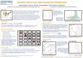
1. Trading space for time in Bayesian framework Nataliya Bulygina1, Susana L. Almeida1, Thorsten Wagener2, Wouter Buytaert1, Neil McIntyre1 1Department of Civil and Environmental Engineering, Imperial College London, UK (n.bulygina@imperial.ac.uk); 2 Department of Civil Engineering, University of Bristol, Bristol, UK ABSTRACT RESULTS: LIKELIHOOD Regionalised information, as contained in regionalised streamflow response indices, is used in a Bayesian framework to constrain hydrological models, thus trading space for time when dealing with non-stationarity. In our approach, likelihoods are derived explicitly by taking account of the inter-index error covariance structure. Meanwhile the prior is shown to play a significant role, and the assumption of uniform parameter priors is found to be unsuitable, and a transformation is required. US catchments taken from the MOPEX database are used to test the methodological development. On average, prediction quality stops improving after including information from a sub-set of indices (three, as shown here). Model structure used appears incapable of capturing sub-sets of behavioural indices. Distribution of α from QQ plots (the closer to α =1 the better) Model inability to represent a pair of indices: modelled distribution of indices vs. regionalised indices (red star) BAYES’ LAW METHOD: PRIOR A model transforms the common uniform-in-parameters prior into a non-uniform-in-output prior, which often illustrates that the highest sampling density is in less relevant parts of the output space. In data-scarce problems (here, using regionalised indices), where the shape of the prior is influential on the posterior, this leads to bias. We propose to use a uniform-in-indices distribution as a prior. Due to numerical sampling difficulties, importance sampling can be used, so that a uniform-in-indices prior p0 approximates as where model parameters Θ are drawn from a proposal distribution g(.), weights wi are inversely proportional to a behavioural index distribution G(.) that is a model M transformation of the proposal distribution g(.). M – model, Θ – model parameters, I*- regionalized indices, IM, Θ– modelled indices, L(IM, Θ | I*) – model parameter likelihood given regionalised indices, and p0(Θ|M) – prior model parameter distribution. METHOD : LIKELIHOOD Five behavioural indices are considered: - Runoff Ratio (RR), - Base Flow Index (BFI), - High Pulse Count (HPC), - Slope of Flow Duration Curve (SFDC), - Streamflow Elasticity (SE). The indices are related to climatic indices, catchment shape characteristics, soils, and vegetation (LAI) via a step-wise regression (Almeida et al, 2012). Probability distributions are fitted to the residuals including inter-index residual covariance, and used to define likelihoods. Uniform-in-parameters prior, likelihood, and resulting posterior pdfs in behavioural index space RESULTS: PRIOR FLOW TIME SERIES INDICES A uniform-in-index prior leads to more consistent predictions of the behavioural indices when compared to uniform-in-parameters prior. Reliability of flow time series predictions is generally better when a uniform-in-index prior is used (orange box plots for α), rather than uniform-in-parameters • CONCLUSIONS • Due to model structural error, more information does not necessarily lead to better predictions. • The prior plays an important role under data-scarce conditions, and can bias predictions due to model choice. • When a few pieces of information are available a prior that is uniform in the relevant output space (not parameters), is recommended to be used in Bayesian conditioning. Distribution across 84 catchments of α from QQ plots (the closer to α =1 the better) REFERENCE Almeida, S., N. Bulygina, N. McIntyre, T. Wagener, and W. Buytaert, 2012. Predicting flows in ungauged catchments using correlated information sources, BHS National Symposium Proceedings, Dundee, UK. Closeness of line to the diagonal reflects consistency of estimated posterior with observed indices Susana Almeida is supported under FCT - Fundação para a Ciência e a Tecnologia, Portugal (grant SFRH/BD/65522/2009).