Hypothesis Testing with Two Populations
Hypothesis Testing with Two Populations. Week 9 GT00303. Comparing 2 Populations. Previously we looked at techniques to estimate and test parameters for one population: Population Mean (µ) Population Variance ( σ 2 )


Hypothesis Testing with Two Populations
E N D
Presentation Transcript
Hypothesis Testing with Two Populations Week 9 GT00303
Comparing 2 Populations Previously we looked at techniques to estimate and test parameters for one population: Population Mean (µ) • Population Variance (σ2) We will still consider these parameters when we are looking at two populations, however our interest will now be: • The difference between two means (µ1- µ2). • The ratio of two variances (σ12 / σ22). 9-2
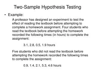
Difference between 2 Means (Independent Samples) In order to test and estimate the difference between two population means, we draw random samples from each of two populations. Initially, we will consider independent samples, that is, samples that are completely unrelated to one another. 9-3
Population 1 Population 2 Sample, size: n1 Sample, size: n2 Statistics: Statistics: Parameters: Parameters: 9-4
The sampling distribution of . • (1) If populations are normal (approximately normal): • (2) If populations are non-normal: 9-5
In practice, the population variances (σ2) are unknown. So, z statistic is rarely used ?? In this case, we have to replace them with sample variances (s), and use t-statistic! 9-6
However, the application of t-test depends on 2 conditions: • When we believe the population variances are equal (equal-variances t-test) • When we believe the population variances are not equal (unequal-variances t-test) 9-7
(1) Equal-variance t-test for (μ1 - μ2) Pooled variance estimator 9-8
(2) Unequal-variance t-test for (μ1 - μ2) When the two population variances are unequal, we cannot pool the data and produce a common estimator. 9-9
So, which t-test to use? Equal-variances or unequal- variances? We have to first test the hypothesis of equal variances! 1st Hypothesis H0: σ12 / σ22 = 1 H1: σ12 / σ22 ≠ 1 2nd Hypothesis H0: µ1- µ2 = 0 H1: µ1- µ2 > 0 If reject H0 and conclude unequal variances, USE unequal-variances t-test for 2nd hypothesis. • If do not reject H0 and conclude insufficient evidence that variances are unequal, USE equal-variances t-test for 2nd hypothesis 9-10
How to test 1st Hypothesis? 1st Hypothesis H0: σ12 / σ22 = 1 H1: σ12 / σ22 ≠ 1 The rejection region and critical value can be obtained from the F-table. 9-11
Illustration 1: Millions of investors buy mutual funds choosing from thousands of possibilities. Some funds can be purchased directly from banks or other financial institutions while others must be purchased through brokers, who charge a fee for this service. This raises the question, can investors do better by buying mutual funds directly than by purchasing mutual funds through brokers. To help answer this question a group of researchers randomly sampled the annual returns from mutual funds that can be acquired directly and mutual funds that are bought through brokers and recorded the net annual returns, which are the returns on investment after deducting all relevant fees. Can we conclude at the 5% significance level that directly-purchased mutual funds outperform mutual funds bought through brokers? 9-12
Population 1 Net annual return from directly-purchased mutual funds Population 2 Net annual return from broker-purchased funds µ1 = mean net annual return for population 1 µ2 = mean net annual return for population 2 9-13
From the data Xm13-01 (click here), we can compute sample mean and sample variance using Excel: Preliminary Test Since population variances (σ2) are unknown, we will use t-distribution. But which t-test to use? Equal-variances or unequal-variances? 9-14
To decide, we apply the F-test on the following hypothesis: H0: σ12 / σ22 = 1 H1: σ12 / σ22 ≠ 1 We will compare this test statistic with the critical value (or rejection region). For F-table, we use α = 5%, and degree of freedom v1 = 50-1 = 49, v2 = 50 – 1 =49. It is a two-tail test. 9-15
Right-tail Critical Value: Left-tail Critical Value: The F-table gives critical value for right-tail test. Because the F distribution is not symmetric, and there are no negative values, you CANNOT simply take the opposite of the right critical value to find the left critical value. The way to find a left critical value is to reverse the degrees of freedom, look up the right critical value, and then take the reciprocal of this value 9-16
The Rejection Region is F < 0.57 F > 1.75 The test statistic of 0.86 does not fall into the Rejection Region. Do not reject H0 and conclude that there is insufficient evidence to infer the population variances are unequal. So, for this illustration, we will conduct the hypothesis testing using equal-variances t-test. 9-17
Step 1: The hypothesis to be tested is that the mean net annual return from directly-purchased mutual funds (µ1) is larger than (outperform) the mean of broker-purchased funds (µ2). • H0: µ1- µ2 = 0 • H1: µ1-µ2 > 0 H0 is presumed to be true This is what we want to prove! 9-18
Step 2: Since population variances (σ2) are unknown, we will use t-distribution. Our F-test earlier suggests the use of equal-variances t-test. Pooled variance estimator 9-19
d.f. = n1 + n2 -2 = 50 + 50 – 2 = 98 9-20
Step 3: With α= 0.05 and it is a one-tail test (right tail), the critical value and rejection region is as follows: 0.05 t0.05,98=??? 9-21
t0.05, 98 = 1.661 9-22
Step 4: Reject H0 if the computed test statistic (from Step 2, t = 2.29) falls into the shaded Rejection Region, or t > 1.661 Step 5: Reject H0 at the 5% level of significance and conclude there is sufficient evidence to infer that on average directly-purchased mutual funds outperform broker-purchased mutual funds. 9-23
Can we estimate the 95% confidence interval for μ1-μ2? It is estimated that the return on directly purchased mutual funds is on average between 0.39and 5.43 percentage points larger than broker-purchased mutual funds. 9-24
Illustration 2: What happens to the family-run business when the boss’s son or daughter takes over? Does the business do better after the change if the new boss is the offspring of the owner or does the business do better when an outsider is made chief executive officer (CEO)? In pursuit of an answer researchers randomly selected 140 firms between 1994 and 2002, 30% of which passed ownership to an offspring and 70% appointed an outsider as CEO. For each company the researchers calculated the operating income as a proportion of assets in the year before and the year after the new CEO took over. Do these data allow us to infer at the 5% level of significance that the effect of making an offspring CEO is different from the effect of hiring an outsider as CEO? 9-25
Population 1: Operating income of companies whose CEO is an offspring of the previous CEO Population 2: Operating income of companies whose CEO is an outsider µ1 = mean operating income for population 1 µ2 = mean operating income for population 2 From the data Xm13-02 (click here), we can compute sample mean and sample variance using Excel: 9-26
Preliminary Test Since population variances (σ2) are unknown, we will use t-distribution. But which t-test to use? Equal-variances or unequal-variances? To decide, we apply the F-test on the following hypothesis: H0: σ12 / σ22 = 1 H1: σ12 / σ22 ≠ 1 9-27
We will compare this test statistic with the critical value (or rejection region). To use the F-table, we use α = 5%, and degree of freedom v1 = 42-1 = 41, v2 = 98 – 1 =97. It is a two-tail test. Right-tail Critical Value: Left-tail Critical Value: 9-28
The Rejection Region is F < 0.57 F > 1.64 The test statistic of 0.47 falls into the Rejection Region. Reject H0 and conclude that there is sufficient evidence to infer the population variances are unequal. So, for this illustration, we will conduct the hypothesis testing using unequal-variances t-test. 9-29
Step 1: The hypothesis to be tested is that the mean operating income for companies whose CEO is an offspring of the previous CEO (µ1) is different from the mean operating income of companies whose CEO is an outsider (µ2). • H0: µ1- µ2 = 0 • H1: µ1-µ2 ≠ 0 H0 is presumed to be true This is what we want to prove! 9-30
Step 2: Since population variances (σ2) are unknown, we will use t-distribution. Our F-test earlier suggests the use of unequal-variances t-test. 9-31
Step 3: With α= 0.05 and it is a two-tail test, the critical value and rejection region is as follows: 0.025 0.025 t0.025,111=??? -t0.025,111=??? 9-33
Step 4: Reject H0 if the computed test statistic (from Step 2, t = -3.22) falls into the shaded Rejection Region, or t < -1.982 t > 1.982 Step 5: Reject H0 at the 5% level of significance and conclude that there is sufficient evidence to infer that mean operating income for the two populations are different. 9-34
Difference between 2 Means (Matched Pairs) Previously, we consider independent samples, that is, samples that are completely unrelated to one another. • When an observation in one sample is matched with an observation in a second sample, this is called a matched pairs experiment. 9-35
Illustration 3A: In the last few years, a number of web-based companies that offer job placement services have been created. The manager of one such company wanted to investigate the job offers recent MBAs were obtaining. In particular, she wanted to know whether finance majors were being offered higher salaries than marketing majors. In a preliminary study she randomly sampled 50 recently graduated MBAs half of whom majored in finance and half in marketing. From each she obtained the highest salary (including benefits) offer. Can we infer at the 5% level of significance that finance majors obtain higher salary offers than do marketing majors among MBAs? 9-36
Population 1 Highest salary offer to finance majors Population 2 Highest salary offer to marketing majors µ1 = mean highest salary offer for population 1 µ2 = mean highest salary offer for population 2 9-37
From the data Xm13-04 (click here), we can compute sample mean and sample variance using Excel: Preliminary Test Since population variances (σ2) are unknown, we will use t-distribution. But which t-test to use? Equal-variances or unequal-variances? 9-38
To decide, we apply the F-test on the following hypothesis: H0: σ12 / σ22 = 1 H1: σ12 / σ22 ≠ 1 We will compare this test statistic with the critical value (or rejection region). To use the F-table, we use α = 5%, and degree of freedom v1 = 25-1 = 24, v2 = 25 – 1 =24. It is a two-tail test. 9-39
Left-tail Critical Value Right-tail Critical Value The Rejection Region is F < 0.44 F > 2.27 The test statistic of 1.37 does not fall into the Rejection Region. Do not reject H0 and conclude that there is insufficient evidence to infer the population variances are unequal. So, for this illustration, we will conduct the hypothesis testing using equal-variances t-test. 9-40
Step 1: The hypothesis to be tested is that the mean highest salary offer for finance majors (µ1) is larger than the mean highest salary offer for marketing majors (µ2). • H0: µ1- µ2 = 0 • H1: µ1-µ2 > 0 H0 is presumed to be true This is what we want to prove! 9-41
Step 2: Since population variances (σ2) are unknown, we will use t-distribution. Our F-test earlier suggests the use of equal-variances t-test. Pooled variance estimator 9-42
d.f. = n1 + n2 -2 = 25 + 25 – 2 = 48 9-43
Step 3: With α= 0.05 and it is a one-tail test (right tail), the critical value and rejection region is as follows: 0.05 t0.05,48=??? 9-44
Step 4: Reject H0 if the computed test statistic (from Step 2, t = 1.04) falls into the shaded Rejection Region, or t > 1.676 Step 5: Do not reject H0 at the 5% level of significance and conclude there is insufficient evidence to infer that finance majors receive higher salary offers than marketing majors. 9-45
Illustration 3B: Suppose now that we redo the experiment in the following way. We examine the transcripts of finance and marketing MBA majors. We randomly sample a finance and a marketing major whose grade point average (GPA) falls between 3.92 and 4 (based on a maximum of 4). We then randomly sample a finance and a marketing major whose GPA is between 3.84 and 3.92. We continue this process until the 25th pair of finance and marketing majors are selected whose GPA fell between 2.0 and 2.08 (The minimum GPA required for graduation is 2.0.) As in Illustration 3A, we recorded the highest salary offer. Can we infer at the 5% level of significance that finance majors obtain higher salary offers than do marketing majors among MBAs? 9-46
In Illustration 3A, the samples are independent. Illustration 3B is a matched pairs experiment, i.e., each observation in one sample is matched with an observation in the other sample. The matching is conducted by selecting finance and marketing majors with similar GPAs. For full data, click here 9-47
For each GPA group (e.g., Group 1 has GPA between 3.92 and 4), we calculate the matched pair difference between the salary offers for finance and marketing majors. The difference of the means is equal to the mean of the differences, hence we will consider the “mean of the paired differences” as our parameter of interest: 9-48
From the data Xm13-05 (click here), we can compute sample mean and sample variance using Excel: Step 1: The hypothesis to be tested is that the mean highest salary offer for finance majors (µ1) is larger than the mean highest salary offer for marketing majors (µ2). • H0: µD = 0 • H1: µD > 0 H0 is presumed to be true This is what we want to prove! 9-49
Step 2: The test statistic for the mean of the population of differences (µD) is: d.f. = nD – 1 = 25 – 1 = 24 9-50