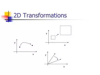
Computer Graphics 2D Transformations

1. Computer Graphics 2D Transformations

2. Contents • In today’s lecture we’ll cover the following: • Why transformations • Transformations • Translation • Scaling • Rotation • Homogeneous coordinates • Matrix multiplications • Combining transformations

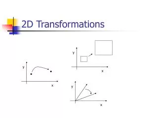
3. Why Transformations? Images taken from Hearn & Baker, “Computer Graphics with OpenGL” (2004) • In graphics, once we have an object described, transformations are used to move that object, scale it and rotate it

4. Translation • A translationis applied to an object by repositioning it along a straight-line path from one coordinate location to another. • We translate a two-dimensional point by adding translationdistances, txand ty, to the original coordinate position (x,y) to move the point to a new position (x′, y′)

5. Translation • The translation distance pair (tx, ty )is called a translationvectoror shiftvector

6. Translation • This allows us to write the two-dimensional translation equations in the matrix form: • where

7. Example y 6 5 4 3 2 1 0 1 2 3 4 5 6 7 8 9 10 x Note: House shifts position relative to origin

8. Scaling • A scalingtransformation alters the size of an object. • This operation can be carried out for polygons by multiplying the coordinate values (x,y) of each vertex by scalingfactorssx, syto produce the transformed coordinates (x′, y′):

9. Scaling • Transformation Equations (Matrix Form): • Or • where S is the 2 by 2 scaling matrix.

10. Scaling • Remarks: • When sxand syare assigned the same value, a uniformscalingis produced that maintains relative object proportions. • Unequal values for sxand syresult in a differentialscalingthat is often used in design applications, where pictures are constructed from a few basic shapes that can be adjusted by scaling and positioning transformations.

11. Example • Turning a square (a) into a rectangle (b) with scaling factors sx = 2 and sy =1.

12. Scaling • When the scaling factors sxand syare assigned the values less than 1, the objects move closer to the coordinate origin. • Similarly, the values of sxand sygreater than 1, move coordinate positions farther from the origin.

13. Example

14. Scaling • When the scaling factors sxand syare assigned the values less than 1, the objects reduce in size. • Similarly, the values of sxand sygreater than 1, enlarge the object size (see Fig. 7). • Warning: Negative values of sxand syare not permissible.

15. Scaling • We can control the location of a scaled object by choosing a position, called the fixedpoint, that is to remain unchanged after the scaling transformation. • Coordinates for the fixed point (xf , yf )can be chosen as one of the vertices, the object centroid , or any other position see next Figure.

16. Example

17. Scaling • Transformation equations, with the fixed point ( xf , yf), are calculated as: • We can rewrite these scaling transformations to separate the multiplicative and the additive terms as follows: (13) (14)

18. Scaling • The additive terms xf (1 - sx) and yf (1-sy) are constant for all points in the object. • Polygons are scaled by applying transformations (14) to each vertex and then regenerating the polygon using the transformed vertices. • Other objects are scaled by applying transformations (14) to the parameters defining the objects. • For example, an ellipse in the standard position is resized by scaling the semi-major and semi-minor axes and redrawing the ellipse about the designated center coordinates.

19. Rotation • The two-dimensional rotationis applied to an object by repositioning it along a circular path in the x-y plane. • To generate a rotation, we specify a rotation angleθ and the position (xr,yr) of the rotation point(or pivot point) about which object is rotated as shown in the Figure.

20. Rotation • This transformation can also be described as a rotation about a rotation axis that is perpendicular to the x-y plane and passes through the pivot point.

21. Rotation • Rotation about the Origin:

22. Rotation • In the previous Figure: • r – is the constant distance of the point from the origin. • is the original angular position of the point from th horizontal • is the rotation angle. • Using the standard trigonometric identities, we can express the transformed coordinates in terms of the two angles as

23. Rotation • The original coordinates of the point in polar coordinates are: • x = r cos φ, y = r sin φ (5) • • Substituting expressions (5) into (4) , we obtain the transformation equations for rotating a point at position (x, y) through and an angle about the origin: x' = x cos θ - y sin θ, y' = x sin θ+ y cos θ (6)

24. Rotation • Rotation Equations in the Matrix Form: • P' = R . P (7) • Where the rotation matrix is

25. Rotation of a point about an arbitrary pivot position is shown bellow:

26. Rotation • Using the trigonometric relationships indicated by the two right triangles in the previous Figue, we can generalize equation (6) to obtain the transformation equations for rotation of a point about any specified rotation position (xr,yr):

27. Rotation • Rotation is a rigid-body transformations that move objects without deformation. • Every point on an object is rotated through the same angle. • A straight line segment is rotated by applying the rotation equation (9) to each of the two line endpoints and redrawing the line between the new endpoint positions.

28. Rotation • A polygon is rotated by displaying each vertex using the specified rotation angle and then generating the polygon using the new vertices. • A curve is rotated by repositioning the defining points for the curve and then redrawing it. • An ellipse is rotated about its center coordinates simply by rotating the major and minor axes.

29. Example y 6 5 4 3 2 1 x 0 1 2 3 4 5 6 7 8 9 10

30. Matrix Representationsand Homogeneous Coordinates • All transformations can be expressed in the following general Matrix Form: • where • P and P′ are column vectors for the coordinate positions. • Matrix M1 is a 2 by 2 array containing multiplicative factors. • Matrix M2 is a 2-element column matrix, containing translational terms factors.

31. Matrix Representationsand Homogeneous Coordinates • More Convenient Method: • Combine the multiplicative and translational terms into a single Matrix Representation, by expanding 2 by 2 Matrix Representation to 3 by 3 matrices.

32. Matrix Representationsand Homogeneous Coordinates • Represent each Cartesian coordinate position (x, y) with homogeneous coordinate triple (xh , yh ,h), • where

33. Matrix Representationsand Homogeneous Coordinates • Thus, a general homogeneous coordinate representation can also be written as (h.x, h.y, h). • h can be selected to be any nonzero value. • Thus, there is an infinite number of equivalent homogeneous representations for each coordinate point (x, y). • A convenient choice is h =1, so that (x, y) becomes (x, y, 1)

34. Matrix Representationsand Homogeneous Coordinates • For Translation • Equation (13) can be expressed as:

35. Matrix Representationsand Homogeneous Coordinates • Or simply • with T (tx ,ty ) as the 3 by 3 translation matrix in Eqn. (15). • Note: The inverse of the translation matrix is obtained by replacing the translation parameters tx and ty with their negatives: -tx and - ty .

36. Matrix Representationsand Homogeneous Coordinates • For Rotation • Equation (13) can be expressed as:

37. Matrix Representationsand Homogeneous Coordinates • Or simply • with R(θ) as 3 by 3 Rotation matrix in Eqn. (17). • Note: The inverse of the Rotation matrix is obtained by replacing the Rotation angle θ with -θ.

38. Matrix Representationsand Homogeneous Coordinates • For Scaling • Equation (13) can be expressed as:

39. Matrix Representationsand Homogeneous Coordinates • Or simply • with S (sx ,sy)as 3 by 3 Scaling matrix in Eqn. (19). • Note: The inverse of the scaling matrix is obtained by replacing the scaling parameters sx and sy with their multiplicative inverses 1/ sx and 1/ sy .

40. Why Homogeneous Coordinates? • All of the transformations can be represented as 3*3 matrices. • The use of matrix multiplication to calculate transformations is efficient.

41. Summary Homogeneous Translation • The translation of a point by (tx ,ty) can be written in matrix form as: • Representing the point as a homogeneous column vector we perform the calculation as:

42. Remember Matrix Multiplication • Recall how matrix multiplication takes place:

43. Summary Homogenous Coordinates • To make operations easier, 2-D points are written as homogenous coordinate column vectors Translation: Scaling:

44. Summary Homogenous Coordinates Rotation:

45. Inverse Transformations • Transformations can easily be reversed using inverse transformations

46. Composite Transformations • With the matrix representations, we can set up matrix for any sequence of transformations as a composite transformation matrix by calculating the matrix product of the individual transformations. • Forming products of transformation matrices is often referred to as a concatenation, or composition of matrices.

47. Composite Transformations • Two successive Translations • where P and P′ are represented as homogeneous coordinate column vectors.

48. Composite Transformations • The composite Transformation matrix is as follows: • Or

49. Composite Transformations • Two successive Rotations • The composite Transformation matrix is as follows:

50. Composite Transformations • so that the final rotated coordinates can be calculated as: