2D TRANSFORMATIONS
2D TRANSFORMATIONS. 2D Transformations. What is transformations? The geometrical changes of an object from a current state to modified state. Why the transformations is needed? To manipulate the initially created object and to display the modified object without having to redraw it.

2D TRANSFORMATIONS
E N D
Presentation Transcript
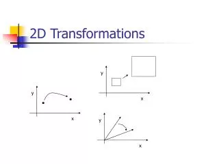
2D Transformations • What is transformations? • The geometrical changes of an object from a current state to modified state. • Why the transformations is needed? • To manipulate the initially created object and to display the modified object without having to redraw it.
2D Transformations • 2 ways • Object Transformation • Alter the coordinates descriptions an object • Translation, rotation, scaling etc. • Coordinate system unchanged • Coordinate transformation • Produce a different coordinate system
a c b d Matrix Math • Why do we use matrix? • More convenient organization of data. • More efficient processing • Enable the combination of various concatenations • Matrix addition and subtraction c a = d b
Matrix Math • How about it? • Matrix Multiplication • Dot product a c d e f b e f g h a b c d a.e + b.g a.f + b.h c.e + d.g c.f + d.h . =
6 6 Matrix Math • What about this? • Type of matrix . 1 2 3 1 1 2 = 1 2 3 1 2 3 . tak boleh!! = a a b b Row-vector Column-vector
+ é ù é ù é ù a b e ae bf · ê ú ê ú ê ú + c d f ce df ë û ë û ë û é ù a b [ ] [ ] · + + e f ae cf be df ê ú c d ë û é ù a c [ ] ] · + + e f ae bf ce df ê ú b d ë û Matrix Math • Is there a difference between possible representations? = = [ =
Matrix Math • We’ll use the column-vector representation for a point. • Which implies that we use pre-multiplication of the transformation – it appears before the point to be transformed in the equation. • What if we needed to switch to the other convention?
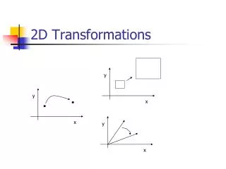
A translation moves all points in an object along the same straight-line path to new positions. The path is represented by a vector, called the translation or shift vector. We can write the components: p'x= px + tx p'y= py + ty or in matrix form: P'= P+T ? =4 ty = 6 tx (2, 2) Translation x’ y’ x y tx ty = +
Rotation • A rotation repositions all points in an object along a circular path in the plane centered at the pivot point. • First, we’ll assume the pivot is at the origin. P’ P
Rotation P’(x’, y’) r y’ P(x,y) r y x x’ Identity of Trigonometry • Review Trigonometry • => cos = x/r , sin = y/r • x = r. cos, y = r.sin • => cos (+ ) = x’/r • x’ = r. cos (+ ) • x’ = r.coscos -r.sinsin • x’ = x.cos – y.sin • =>sin (+ ) = y’/r y’ = r. sin (+ ) • y’ = r.cossin + r.sincos • y’ = x.sin + y.cos
Rotation • We can write the components: • p'x = px cos – py sin • p'y= px sin + py cos • or in matrix form: • P' = R •P • can be clockwise (-ve) or counterclockwise (+ve as our example). • Rotation matrix P’(x’, y’) y’ P(x,y) r y x x’
Rotation • Example • Find the transformed point, P’, caused by rotating P= (5, 1) about the origin through an angle of 90.
Scaling P’ P • Scaling changes the size of an object and involves two scale factors, Sx and Sy for the x- and y- coordinates respectively. • Scales are about the origin. • We can write the components: • p'x = sx•px • p'y = sy•py • or in matrix form: • P' = S •P • Scale matrix as:
Scaling • Example : • P(2, 5), Sx = 0.5, Sy = 0.5 • Find P’ ? P(2, 5) P’ • If the scale factors are in between 0 and 1 the points will be moved closer to the origin the object will be smaller.
Scaling P’ • Example : • P(2, 5), Sx = 0.5, Sy = 0.5 • Find P’ ? P(2, 5) P’ • Example : • P(2, 5), Sx = 2, Sy = 2 • Find P’ ? • If the scale factors are in between 0 and 1 the points will be moved closer to the origin the object will be smaller. • If the scale factors are larger than 1 the points will be moved away from the origin the object will be larger.
Scaling P’ P(1, 2) • If the scale factors are the same, Sx = Sy uniform scaling • Only change in size (as previous example) • If Sx Sy differential scaling. • Change in size and shape • Example : square rectangle • P(1, 3), Sx = 2, Sy = 5 , P’ ? What does scaling by 1 do? What is that matrix called? What does scaling by a negative value do?
Combining transformations We have a general transformation of a point: P' = M•P + A When we scale or rotate, we set M, and A is the additive identity. When we translate, we set A, and M is the multiplicative identity. To combine multiple transformations, we must explicitly compute each transformed point. It’d be nicer if we could use the same matrix operation all the time. But we’d have to combine multiplication and addition into a single operation.
Homogenous Coordinates y y w x • Let’s move our problem into 3D. • Let point (x, y) in 2D be represented by point (x, y, 1) in the new space. • Scaling our new point by any value a puts us somewhere along a particular line: (ax, ay, a). • A point in 2D can be represented in many ways in the new space. • (2, 4) ---------- (8, 16, 4) or (6, 12, 3) or (2, 4, 1) or etc. x
Homogenous Coordinates • We can always map back to the original 2D point by dividing by the last coordinate • (15, 6, 3) --- (5, 2). • (60, 40, 10) - ?. • Why do we use 1 for the last coordinate? • The fact that all the points along each line can be mapped back to the same point in 2D gives this coordinate system its name – homogeneous coordinates.
Matrix Representation x y 1 • Point in column-vector: • Our point now has three coordinates. So our matrix is needs to be 3x3. • Translation
Matrix Representation • Rotation • Scaling
Composite Transformation • We can represent any sequence of transformations as a single matrix. • No special cases when transforming a point – matrix • vector. • Composite transformations – matrix • matrix. • Composite transformations: • Rotate about an arbitrary point – translate, rotate, translate • Scale about an arbitrary point – translate, scale, translate • Change coordinate systems – translate, rotate, scale • Does the order of operations matter?
æ ö + + é ù é ù é ù é ù é ù a b e f i j ae bg af bh i j ç ÷ · · = · ê ú ê ú ê ú ê ú ê ú ç ÷ + + c d g h k l ce dg cf dh k l ë û ë û ë û ë û ë û è ø + + + + + + é ù aei bgi afk bhk aej bgj afl bhl = ê ú + + + + + + cei dgi cfk dhk cej dgj cfl dhl û ë æ ö + + é ù é ù é ù é ù é ù a b e f i j a b ei fk ej fl ç ÷ · · = · ê ú ê ú ê ú ê ú ê ú ç ÷ + + c d g h k l c d gi hk gj hl ë û ë û ë û ë û ë û è ø + + + + + + é ù aei afk bgi bhk aej afl bgj bhl = ê ú + + + + + + cei cfk dgi dhk cej cfl dgj dhl ë û Composition Properties ? • Is matrix multiplication associative? • (A.B).C = A.(B.C)
Composition Properties ? • Is matrix multiplication commutative? • A . B = B . A
Order of operations So, it does matter. Let’s look at an example: • Rotate • Translate • Translate • Rotate
Composite Transformation Matrix cos -sin 0 sin cos 0 0 0 1 1 0 tx 0 1 ty 0 0 1 1 0 -tx 0 1 -ty 0 0 1 . . cos -sin -tx cos+ ty sin sin cos -tx sin - ty cos 0 0 1 1 0 tx 0 1 ty 0 0 1 . cos -sin -tx cos+ ty sin + tx sin cos -tx sin - ty cos + ty 0 0 1 • Arrange the transformation matrices in order from right to left. • General Pivot- Point Rotation • Operation :- • Translate (pivot point is moved to origin) • Rotate about origin • Translate (pivot point is returned to original position) T(pivot) • R() • T(–pivot)
x y 1 . 2 5 1 0.5 -0.866 -1.0.5 + 2.0.866 + 1 0.866 0.5 -1.0.866- 2.0.5 + 2 0 0 1 . 2 5 1 -1.098 4.366 1 0.5 - 0.866 2.232 0.866 0.5 0.134 0 0 1 . = cos -sin -tx cos+ ty sin+ tx sin cos -tx sin - ty cos + ty 0 0 1 Composite Transformation Matrix • Example • Perform 60 rotation of a point P(2, 5) about a pivot point (1,2). Find P’? Sin 60 = 0.8660 Kos 60 = 1/2 P’ = (-1, 4)
Without using composite homogenus matrix • Example • Perform 90 rotation of a point P(5, 1) about a pivot point (2, 2). Find P’? • 1. Translate pivot point ke asalan ( tx = -2, ty = -2) • Titik P(5, 1 ) P’ (3, -1) • 2. Rotate P ‘ = 90 degree • P’(3, -1) -- > kos 90 -sin 90 3 = 0 -1 3 = 1 • sin 90 kos 90 -1 1 0 -1 3 • 3. Translate back ke pivot point (tx = 2 , ty = 2) • titik (1, 3 ) titik akhir (3, 5)
Composite Transformation Matrix • General Fixed-Point Scaling • Operation :- • Translate (fixed point is moved to origin) • Scale with respect to origin • Translate (fixed point is returned to original position) T(fixed) • S(scale) • T(–fixed) Find the matrix that represents scaling of an object with respect to any fixed point? Given P(6, 8) , Sx = 2, Sy = 3 and fixed point (2, 2). Use that matrix to find P’?
Answer Sx 0 0 0 Sy 0 0 0 1 1 0 tx 0 1 ty 0 0 1 1 0 -tx 0 1 -ty 0 0 1 . . Sx 0 -tx Sx 0 Sy -ty Sy 0 0 1 1 0 tx 0 1 ty 0 0 1 Sx 0 -tx Sx + tx 0 Sy -ty Sy + ty 0 0 1 = . x =6, y = 8, Sx = 2, Sy = 3, tx =2, ty = 2 2 0 -2(2) + 2 0 3 -2(3) + 2 0 0 1 6 8 1 10 20 1 . =
Composite Transformation Matrix General Scaling Direction Operation :- 1. Rotate (scaling direction align with the coordinate axes) 2. Scale with respect to origin 3. Rotate (scaling direction is returned to original position) R(–) • S(scale) • R() Find the composite transformation matrix by yourself !!
latihan • Dapatkan titik akhir bagi P(5, 8) jika titik tersebut diputarkan sebanyak 90 darjah, kemudian ditranslate sebanyak (-6, 9) dan akhirnya diskala dengan faktor skala (2, 0.5).
S . T . R Sx 0 0 0 Sy 0 0 0 1 cos -sin 0 sin cos 0 0 0 1 1 0 tx 0 1 ty 0 0 1 . . Sx 0 0 0 Sy 0 0 0 1 cos -sin tx sin cos ty 0 0 1 . Sxcos Sx(-sin) Sx tx Sy sin Sy cos Sy ty 0 0 1
Other transformations Reflection: x-axis y-axis
Other transformations Reflection: origin line x=y
Other transformations Shear: x-direction y-direction
Coordinate System Transformations • We often need to transform points from one coordinate system to another: • We might model an object in non-Cartesian space (polar) • Objects may be described in their own local system • Other reasons: textures, display, etc