Download

1 / 36
360 likes | 450 Views
Sinéad M. Farrington University of Liverpool for the CDF and D0 Collaborations Beauty 05 21 st June 2005. Rare Decays at the Tevatron. Outline. Overall motivations B d,s m + m - Motivation CDF and D0 methods CDF and D0 results B d,s m + m - K + /K*/ f Motivation

E N D
Sinéad M. Farrington University of Liverpool for the CDF and D0 Collaborations Beauty 05 21st June 2005 Rare Decays at the Tevatron
Outline • Overall motivations • Bd,s m+m- • Motivation • CDF and D0 methods • CDF and D0 results • Bd,s m+m-K+/K*/f • Motivation • D0 sensitivity analysis For discussion of Charmless B decays see following talk by Simone Donati 0 0 2
l+ Z* c02 q l- q c01 q c+ l+ W+ n • Two ways to search for new physics: • direct searches – seek e.g. Supersymmetric particles • indirect searches – test for deviations from Standard Model predictions e.g. branching ratios • In the absence of evidence for new physics • set limits on model parameters Searching for New Physics BR(Bmm)<1x10⁻⁷ Trileptons: 2fb-1 3
Bd,sm+m- 0 4
In Standard Model FCNC decay B mm heavily suppressed • Standard Model predicts B mm in the Standard Model A. Buras Phys. Lett. B 566,115 • Bd mm further suppressed by CKM coupling (Vtd/Vts)2 • Both below sensitivity of Tevatron experiments Observe no events set limits on new physics Observe events clear evidence for new physics 5
m b RPV SUSY ~ n l’i23 l i22 m s • SUSY could enhance BR by orders of magnitude • MSSM: BR(B mm) tan6b • may be 100x Standard Model B mm in New Physics Models • R-parity violating SUSY: tree level diagram via sneutrino • observe decay for low tan b • mSUGRA: B mm search complements direct SUSY searches • Low tan b observation of trilepton events • High tan b observation of B mm • Or something else! A. Dedes et al, hep-ph/0207026 6
The Challenge search region • Large combinatorial background • Key elements are • determine efficiencies • select discriminating variables • estimate background 7
Search for muon pairs in Bd/Bs mass windows • D0 search for only Bs and correct for Bd decays • Approximately 360pb-1(CDF) /300pb-1(D0) integrated luminosity • Unbiased optimisation, signal region blind • Aim to measure BR or set limit • Reconstruct normalisation mode (B+J/y K+) • Construct discriminant to select B signal and suppress dimuon background (CDF) • Use cuts analysis to suppress dimuon background (D0) • Measure background • Measure the acceptance and efficiency ratios Methodology 8
six dedicated rare B triggers • using all chambers to |h|1.1 • excellent tracking • Use two types of muon pairs: central-central central-extension • four dedicated rare B triggers • using all chambers to |h|2.0 • excellent muon coverage CDF D0 Central Muon Extension (0.6< |h| < 1.0) Central Muon Chambers (|h| < 0.6) Muon Chambers (|h| < 2.0) 9
Normalisation Mode (CDF) • Reconstruct normalisation mode (B+J/y K+) central-central muons 10
cut cut B mm Optimisation (CDF) • Chosen three primary discriminating variables: • proper decay length (l) • Pointing (Da) |fB – fvtx| • Isolation (Iso) 11
signal background B mm Optimisation (D0) • Similar three primary discriminating variables • D0 use 2d lifetime variables instead of 3d • Optimise using MC for signal, data sidebands for background • Random grid search, optimising for 95% C.L. 12
Likelihood Ratio Discriminant (CDF) • First iteration of analysis used standard cuts optimisation • Second iteration uses the more powerful likelihood discriminant • i: index over all discriminating variables • Psig/bkg(xi): probability for event to be signal / background for a given measured xi • Obtain probably density functions of variables using • background: Data sidebands • signal: Pythia Monte Carlo sample 13
Optimisation (CDF) Likelihood ratio discriminant: Optimise likelihood and pt(B) for best 90% C.L. limit • Bayesian approach • consider statistical and systematic errors • Assume 1fb-1 integrated luminosity 14
Expected Background (CDF/D0) • Extrapolate from data sidebands to obtain expected events • CDF: • Scale by the expected rejection from the likelihood ratio cut • Expected background: 0.81 ± 0.12 (central-central dimuon) 0.66 ± 0.13 (central-extended dimuon) • Tested background prediction in several control regions and find good agreement • D0: • Expected background: 4.3 1.2 15
Unblinded Results (D0) • Apply optimised cuts • Unblinded results for Bsmm: • Expected background:4.3 1.2 • Observed: 4 BR(Bsmm) < 3.0×10⁻⁷ @ 90% CL < 3.7×10⁻⁷ @ 95% CL 16
Unblinded Results (CDF) Results with pt(B)>4GeV cut applied, Likelihood cut at 0.99: No events found in Bs or Bd search windows in either muon pair type 17
now Limits on BR(Bd,smm) (CDF) • BR(Bsmm) < 1.6×10⁻⁷ @ 90% CL • < 2.1×10⁻⁷ @ 95% CL • BR(Bdmm) < 3.9×10⁻⁸ @ 90% CL • < 5.1×10⁻⁸ @ 95% CL • These are currently world best limits • The future for CDF: • use optimisation for 1fb-1 • need to reoptimise at 1fb-1 for • best results • assume linear background • scaling 18
Bd,smm K+/K*/f 0 19
B Rare Decays • B+ mm K+ • B0mm K* • Bsmmf • Lbmm L • FCNC b sg* • Penguin or box processes in the Standard Model: • Rare processes: Latest Belle measurement Bd,smm K+/K*/f hep-ex/0109026, hep-ex/0308042, hep-ex/0503044 observed at Babar, Belle m m m m x10-7 20
1) Would be first observations in Bs and Lb channels 2) Tests of Standard Model • branching ratios • kinematic distributions (with enough statistics) • Effective field theory for b s (Operator Product Expansion) • Rare decay channels are sensitive to Wilson coefficients which are calculable for many models (several new physics scenarios e.g. SUSY, technicolor) • Decay amplitude: C9 • Dilepton mass distribution: C7, C9 • Forward-backward asymmetry: C10 Motivations 21
Use B J/yX channels as control channels • exactly the same signature (J/ymm) • use MC to obtain relative efficiency • Most likely confirm observation B+ mm K+ and measure BR • Then either • make first observations in Bs and Lb or • set strong branching ratio limits Analysis Outline (CDF,D0) Bs J/y f 22
Cuts analysis using same variables as Bsmm analysis Sensitivity Analysis (D0) • Remove the dimuon mass regions corresponding to J/y, y’, f • Contribution from rare decays not well understood under resonances 23
Sensitivity Analysis (D0) • Box is unopened • Expected background: 5.1 ± 1.0 events • Sensitivity for 90% C.L. limit calculated: BR(Bsmmf)<1.2 x10⁻⁵ 24
mSUGRA Summary • Bd,sm+m- are a powerful probe of new physics • Could give first hint of new physics at the Tevatron • World best limits coming from Tevatron experiments • Combinations of D0 and CDF results by Lepton Photon 05 SO(10) • Bd,sm+m- K/K*/f should be observable in Run II • Also a test of the Standard Model • Sensitivity analysis performed, awaiting results 25
Backup 26
Dedicated rare B triggers • in total six Level 3 paths • Two muons + other cuts • using all chambers to |h|1.1 • Use two types of dimuons: CMU-CMU CMU-CMX • Additional cuts in some triggers: • Spt(m)>5 GeV • Lxy>100mm • mass(m m)<6 GeV • mass(m m)>2.7 GeV Samples (CDF) 27
LH CMU-CMU CMU-CMX cut pred obsv pred obsv >0.50 236+/-4 235 172+/-3 168 OS- >0.90 37+/-1 32 33+/-1 36 >0.99 2.8+/-0.2 2 3.6+/-0.2 3 >0.50 2.3+/-0.2 0 2.8+/-0.3 3 SS+ >0.90 0.25+/-0.03 0 0.44+/-0.04 0 >0.99 <0.10 0 <0.10 0 >0.50 2.7+/-0.2 1 3.7+/-0.3 4 SS- >0.90 0.35+/-0.03 0 0.63+/-0.06 0 >0.99 <0.10 0 <0.10 0 >0.50 84+/-2 84 21+/-1 19 FM+ >0.90 14.2+/-0.4 10 3.9+/-0.2 3 >0.99 1.0+/-0.1 2 0.41+/-0.03 0 Background estimate (CDF) 1.) OS- : opposite-charge dimuon, l < 0 2.) SS+ : same-charge dimuon, l > 0 3.) SS- : same-charge dimuon, l < 0 4.) FM : fake muon sample (at least one leg failed muon stub chi2 cut) 28
Likelihood p.d.f.s (CDF) Input p.d.f.s: Likelihood ratio discriminant: 29
Methodology (CDF) • Search for muon pairs in Bd/Bs mass windows • D0 search for only Bs and correct for Bd decays • Approximately 360pb-1 integrated luminosity • Blind analysis • Aim to measure BR or set limit • Reconstruct normalization mode (B+J/y K+) • Construct discriminant to select B signal and suppress dimuon background • Measure background • Measure the acceptance and efficiency ratios 30
Signal and Side-band Regions • Use events from same triggers for • B+ and Bs(d) mm reconstruction. • Search region: • - 5.169 < Mmm < 5.469 GeV • - Signal region not used in • optimization procedure s(Mmm)~24MeV Monte Carlo Search region • Sideband regions: • - 500MeV on either side of search region • - For background estimate and analysis • optimization.
MC Samples • Pythia MC • Tune A • default cdfSim tcl • realistic silicon and beamline • pT(B) from Mary Bishai • pT(b)>3 GeV && |y(b)|<1.5 • Bsm+m- • (signal efficiencies) • B+JK+m+m-K+ (nrmlztn efncy and xchks) • B+Jp+m+m-p+ (nrmlztn correction)
SO(10) Unification Model R. Dermisek et al., hep-ph/0304101 • tan(b)~50 constrained by unification • of Yukawa coupling • All previously allowed regions (white) • are excluded by this new measurement • Unification valid for small M1/2 • (~500GeV) • New Br(Bsmm) limit strongly • disfavors this solution for • mA= 500 GeV h2>0.13 mh<111GeV m+<104GeV Excluded by this new result Red regions are excluded by either theory or experiments Green region is the WMAP preferred region Blue dashed line is the Br(Bsmm) contour Light blue region excluded by old Bsmm analysis
Method: Likelihood Variable Choice Prob(l) = probability of Bsmm yields l>lobs (ie. the integral of the cumulative distribution) Prob(l) = exp(-l/438 mm) • yields flat distribution • reduces sensitivity to • MC modeling inaccuracies • (e.g. L00, SVX-z)
Method:Checking MC Modeling of Signal LH • For CMU-CMX: • MC reproduces Data • efficiency vs LHood cut • to 5% or better • Assign 5% (relative) • systematic for • CMU-CMX
Step 4: Compute Acceptance and Efficiencies • Most efficiencies are determined directly from data using inclusive • J/ymm events. The rest are taken from Pythia MC. • a(B+/Bs)= 0.297 +/- 0.008 (CMU-CMU) • = 0.191 +/- 0.006 (CMU-CMX) • eLH(Bs): ranges from 70% for LH>0.9 to • 40% for LH>0.99 • etrig(B+/Bs) = 0.9997 +/- 0.0016 (CMU-CMU) • = 0.9986 +/- 0.0014 (CMU-CMX) Red = From MC Green = From Data Blue = combination of MC and Data • ereco-mm(B+/Bs) = 1.00 +/- 0.03 (CMU-CMU/X) • evtx(B+/Bs) = 0.986 +/- 0.013 (CMU-CMU/X) • ereco-K(B+) = 0.938 +/- 0.016 (CMU-CMU/X)