Objectives: Error Bounds Complexity Theory PAC Learning PAC Bound Margin Classifiers
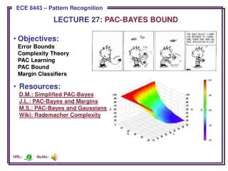
LECTURE 27: PAC-BAYES BOUND. Objectives: Error Bounds Complexity Theory PAC Learning PAC Bound Margin Classifiers Resources: D.M.: Simplified PAC-Bayes J.L.: PAC-Bayes and Margins M.S.: PAC-Bayes and Gaussians Wiki: Rademacher Complexity. Audio:. URL:. Review. Generalized Risk:

Objectives: Error Bounds Complexity Theory PAC Learning PAC Bound Margin Classifiers
E N D
Presentation Transcript
LECTURE 27: PAC-BAYES BOUND • Objectives:Error BoundsComplexity TheoryPAC LearningPAC BoundMargin Classifiers • Resources:D.M.: Simplified PAC-BayesJ.L.: PAC-Bayes and MarginsM.S.: PAC-Bayes and GaussiansWiki: Rademacher Complexity Audio: URL:
Review • Generalized Risk: • Essentially a weighted probability of error. • Fundamental concept in statistical learning theory. • Bayes Risk: the best performance that can be achieved (for the given data set or problem definition). • A useful theoretical abstraction, but difficult to apply in practice. • Chernoff Bound: an approximate bound on the probability of error. • Originally a bound on the probability that a random variable would exceed a given threshold. • Applied to many problems, including calculation of P(E). • Bhattacharyya Bound: a looser but computationally simpler bound. • Risk vs. Empirical Risk: • We were able to develop learning algorithms such as support vector machines and other margin classifiers from this bound. where
Probably Approximately Correct (PAC) Learning1 • We want to learn the concept "medium-built person" from examples. We are given the height and weight of n individuals, the training set. • We want to know which value of n to use if we want to learn this concept well. Our concern is to characterize what we mean by well or good when evaluating learned concepts. • We would like the probability of error of the learned concept to be . • For a specific learning algorithm, what is the probability that a concept it learns will have an error that is bound by epsilon? We would like to set a bound, , on the probability that P(E) : P[P(E) ] <. • This is essentially a confidence measure. We are now in a position to say when a learned concept is good. • Different degrees of "goodness" will correspond to different values of and . • The smaller and are, the better the leaned concept will be. • This method of evaluating learning is called Probably Approximately Correct (PAC) Learning. • We seek a bound on PAC learning for Bayesian estimation. • 1, G. Ingargiola, http://www.cis.temple.edu/~ingargio/cis587/readings/pac.html
Formal Definition of PAC Learning • Definitions: • f is the target function that we desire to learn • F is the class of functions from whichfcan be selected:f F. • Xis the set of possible feature vectors or measurements. • N is the cardinality of X. • Dis a probability distribution on X; this distribution is used both when the training set is created and when the test set is created. • ORACLE(f,D) is a function that in a unit of time returns a pair of the form (x,f(x)), wherexis selected from Xaccording to D. • His the set of possible hypotheses; h, where h H , is the specific hypothesis that has been learned. • nis the cardinality of the training set. • A class of functions F is Probably Approximately (PAC) learnable if there is a learning algorithm, L, that for all f F, all distributions D on X, all and in the range [0,1], will produce an hypothesis h, such that P(E) : P[P(E) ] <. • Fis efficiently PAC learnable if Lis polynomial in , , and log(N). • F is polynomial PAC learnable if n is polynomial in , , and the size of (minimal) descriptions of individuals and of the concept.
PAC Bounds • D. McAllester derived a bound on the generalization error of a PAC learner that is independent of any assumptions about the distribution of the data. This is referred to as a PAC bound. • Early bounds have relied on covering number computations (e.g., VC dimension and empirical risk), while later bounds have considered Rademacher complexity. • Rademacher complexity measures richness of a class of real-valued functions with respect to a probability distribution. • The tightest bounds for practical applications appear to be the PAC-Bayes bound. These bounds are especially attractive for margin classifiers such as SVM, and classifiers built for Gaussian processes. • A PAC bound has to hold independent of correctness of prior knowledge. It does not have to be independent of prior knowledge. • Unfortunately, most standard VC bounds are only vaguely dependent on prior/model they are applied to and lack tightness. • The Bayes classifier integrates over the priors, which is often not tractable. • A Gibbs classifier draws a single sample from the posterior distribution for the class label and uses that as the class assignment. Error at most twice that of the optimal Bayesian classifier.
PAC Bayesian Theorem • For Gibbs classifier: • Assume the prior, P(w), is independent of algorithm, L.. • The posterior, Q(w), may depend on L. • Expected generalization error: • Expected empirical error: • McAllester (1999) showed: • where D() is the divergence (Kullback-Leibler distance), and DBer is the divergence between two Bernoulli distributions with probability of success q and p:
Applying the PAC Bound • Applying the PAC-Bayes bound requires some amount of specialization. • Typically, we specialize to classifiers of the form • We also generally are interested in margin classifiers that use kernels, and not surprisingly, support vector machines are a major area of investigation. • The specializations often include: • The cumulative distribution of a Gaussian: • A posterior distribution, Q(w, µ), that is N(µ,1) for some µ > 0 in the direction of w and N(0,1) in all perpendicular directions. • The normalized margin of the examples: • A stochastic error rate: • To better understand this quantity, consider the case as μ approaches infinity. When the margin is negative (indicating an incorrect classification),approaches 1. • When the margin is positiveapproaches 0. • Thus,is a softened form of the empirical error which takes into account the margin. • Under these assumptions, we can derive a corollary to the PAC-Bayes Theorem describing properties of a PAC-Bayes margin bound.
PAC-Bayes Margin Bound • For all distributions, D, for all [0,1]: • Using the corollary, the true error bound satisfies the equation: • This is an implicit equation for which can be easily solved numerically. • The bound is stated in terms of dot products here, so naturally it is possible to apply kernels, and hence can be applied to SVM learning: • Since, by assumption, k() is a kernel, we know that where() is some projection into another space. • We also note:
Calculation of the Normalized Margin • We can now calculate the normalized margin: • We still need to calculate the mean, µ. • The bound can be nonmonotonic in the value of µ. • For classifiers learned by support vector machines on reasonable datasets, there is only one value of µ which is (locally, and thus globally) minimal. • A binary search can be used to find µ. • But the bound holds for all values of µ simultaneously. • The computational time of the bound calculation is dominated by the calculation of the margins which is O(n2) where n is the number of support vectors with a nonzero associated . • This computational time is typically dominated by the time of the SVM learning algorithm (training).
Summary • Reviewed the concept of error bounds and their importance to pattern recognition. • Introduced Probably Approximately Correct (PAC) learning. • Formally defined PAC learning. • Introduced a theorem that describes a bound on generalization error. • Discussed application of the bound to real problems. • Applied the bound to margin classifiers and showed how it can be used to compute the margin.

