Download
1 / 8
80 likes | 175 Views
Learn about linear, quadratic, cubic, quartic, and quintic functions with positive or negative slopes, roots, and maximums/minimums. Discover how to identify roots, double roots, and draw these functions graphically.

E N D
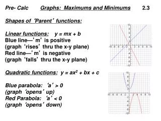
Pre- Calc Graphs: Maximums and Minimums 2.3 Shapes of ‘Parent’ functions: Linear functions: y = mx + b Blue line—’m’ is positive (graph ‘rises’ thru the x-y plane) Red line—’m’ is negative (graph ‘falls’ thru the x-y plane) Quadratic functions: y = ax2 + bx + c Blue parabola: ‘a’ > 0 (graph ‘opens’ up) Red Parabola: ‘a’ < 0 (graph ‘opens’ down)
Cubic graphs: Will have a total of ‘3’ roots y = ax3 + bx2 + cx + d When ‘a’ > 0 (Graph ‘rises’ thru the x-y plane) When ‘a’ < 0 (Graph ‘falls’ thru the x-y plane.)
Quartic functions: Will have a total of ‘4’ roots y = ax4 + bx3 + cx2 + dx + ‘k’ Graph ‘opens’ up ‘a’ > 0 Graph ‘opens’ down ‘a’ < 0
Quintic functions: Will have a total of ‘5’ roots y = ax5 + bx4 + cx3 + dx2 + ex + ‘k’ When ‘a’ > 0 Graph ‘rises’ thru the x-y plane When ‘a’ < 0 Graph ‘’falls’ thru the x-y plane
Knowledge: A graph will always cross the x-axis at its roots! To find the roots, set the ‘rule’ = 0 When a ‘root’ appears once, the graph will pass thru the axis at that value. i.e. the curve will go from below the x-axis to above the x-axis (or vice-versa). Example y = (x-3)(x+2)(x+5) the roots are: x = 3, x = -2, & x = -5 (all ‘single’ roots) (The ‘a’ value would be +1 so this graph rises thru the x-y plane) If a root appears twice it is called a double root. At a ‘double root’, the curve will ‘turn’—(a vertex??)—i.e. that will cause the curve to be tangent to the x-axis at that root. This will be a ‘maximum’ or ‘minimum’ value of the graph.
Example of ‘double roots’: y = (x-3)2(x+4)(x-1) ‘roots’: x = 3, x = - 4, and x = 1, but x = 3 came from the ‘squared’ quantity. Therefore there could have been two (x-3) factors. So x = 3 could have appeared twice Which is why x = 3 is called a ‘double’ root. On the graph when x = 3, the graph turns!
Example: sketch the graph of this factored cubic function: f(x) = (x+1)(x-1)(x-2) 1st: Determine the ‘a’ value simply take (x)(x)(x) = x3 2nd:: find all roots x = - 1, x = 1, x = 2 3rd:: find the y-intercept Need to find the constant simply take (1)(-1)(-2) = 2 4th: Perform a ‘sign analysis’ of f(x) ‘y’ by testing values that lie in between your roots. pick values in between your ‘roots’, plug them in to the equation to find the ‘sign’ of the corresponding ‘y’ values to help you determine whether your graph is either above or below the x-axis in between the roots, 5th: Draw your curve!
The effects of a ‘cube’ root or a ‘fourth’ root A ‘cube’ root causes your graph to ‘flatten’ out as it passes thru the ‘root’. A ‘fourth’ root also causes your graph to ‘flatten’ out but like a ‘double’ root your graph will also turn at that spot.! Example: y = (x – 3)3(x + 4)4 Sketch the graph