Download
1 / 55
670 likes | 954 Views
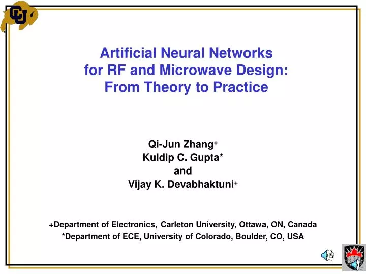
Artificial Neural Networks for RF and Microwave Design: From Theory to Practice. Qi-Jun Zhang + Kuldip C. Gupta* and Vijay K. Devabhaktuni + +Department of Electronics, Carleton University, Ottawa, ON, Canada *Department of ECE, University of Colorado, Boulder, CO, USA. Outline.

E N D
Artificial Neural Networksfor RF and Microwave Design:From Theory to Practice Qi-Jun Zhang+ Kuldip C. Gupta* and Vijay K. Devabhaktuni+ +Department of Electronics,Carleton University, Ottawa, ON, Canada *Department of ECE, University of Colorado, Boulder, CO, USA
Outline • Introduction and overview • Neural network structures • Neural network model development process • RF/Microwave component modeling using neural networks • High-frequency circuit optimization using neural network models • Conclusions
Introduction • Accurate RF/Microwave design is crucial for the current upsurge in VLSI, telecommunication and wireless technologies • Design at microwave frequencies is significantly different from low-frequency and digital designs • Substantial development in RF/microwave CAD techniques have been made during the last decade • Further advances in CAD are needed to address new design challenges, e.g., 3D-EM optimization, CPW and multi-layered circuits, IC antenna modules, etc • Fast and accurate models are key to efficient CAD • Neural network based modeling and design could significantly impact high-frequency CAD
A Quick Illustration Example:Neural Network Model for Delay Estimation in a High-SpeedInterconnect Network
Receiver 1 Driver 1 Driver 2 Receiver 4 Driver 3 Receiver 3 Receiver 2 • High-Speed VLSI • Interconnect Network
R3 C3 • Circuit Representation of the • Interconnect Network 3 L3 L1 1 L2 2 Rs L4 R1 C1 R2 C2 Source Vp, Tr 4 R4 C4
A PCB contains large number of interconnect networks, each with different interconnect lengths, terminations, and topology, leading to need of massive analysis of interconnect networks During PCB design/optimization, the interconnect networks need to be adjusted in terms of interconnect lengths, receiver-pin load characteristics, etc, leading to need of repetitive analysis of interconnect networks This necessitates fast and accurate interconnect network models and neural network model is a good candidate Need for a Neural Network Model
Neural Network Model for Delay Analysis 1 23 4 …... L1 L2 L3 L4 R1 R2 R3 R4 C1 C2 C3 C4 Rs Vp Tr e1 e2 e3
Method CPU Circuit Simulator (NILT) 34.43 hours AWE 9.56 hours Neural Network Approach 6.67 minutes Simulation Time for 20,000 Interconnect Configurations
Neural networks have the ability to model multi-dimensional nonlinear relationships Neural models are simple and the model computation is fast Neural networks can learn and generalize from available data thus making model development possible even when component formulae are unavailable Neural network approach is generic, i.e., the same modeling technique can be re-used for passive/active devices/circuits It is easier to update neural models whenever device or component technology changes Important Features of Neural Networks
Neural models are efficient alternatives to closed-form expressions, equivalent circuit models and look-up tables Neural network models can be developed from measured or simulated data Neural models can also be used to update or improve the accuracy of already existing models Neural network models have been developed for active devices, passive components and interconnect networks These models have been used in circuit simulators for circuit-level simulation, design and optimization Neural Networks for RF/Microwave Applications: Overview
A neural network contains neurons (processing elements) connections (links between neurons) A neural network structure defines how information is processed inside a neuron how the neurons are connected Examples of neural network structures multi-layer perceptrons (MLP) radial basis function (RBF) networks wavelet networks recurrent neural networks knowledge based neural networks MLP is the basic and most frequently used structure Neural Network Structures
y2 y1 ym 1 2 NL (Output)Layer L . . . . 1 2 3 NL-1 (Hidden) Layer L-1 . . . . . . . . . . . (Hidden)Layer 2 1 2 3 N2 . . . . 1 2 3 N1 (Input) Layer 1 . . . . x1 x2 x3 xn MLP Structure
(.) …. Information Processing In a Neuron
Input layer neurons simply relay the external inputs to the neural network Hidden layer neurons have smooth switch-type activation functions Output layer neurons can have simple linear activation functions Neuron Activation Functions
Activation Functions for Hidden Neurons Sigmoid ()=1/(1 +e-) Arc-tangent ()=(2/)arctan() Hyperbolic-tangent ()=(e+ -e-)/(e+ +e-)
y y2 y1 ym z(L) 1 2 NL (Output)Layer L . . . . z(l -1) 1 2 3 NL-1 (Hidden) Layer L-1 . . . . . . . . . . . z(2) (Hidden)Layer 2 1 2 3 N2 . . . . z(1) 1 2 3 N1 (Input) Layer 1 . . . . x x1 x2 x3 xn MLP Structure
Outputs y1 y2 yj =S W ’jkZk k W ’jk Hidden Neuron Values Z1 Z2 Z3 Z4 Zk= tanh(S Wki xi ) i Wki x1 x2 x3 Inputs 3 Layer MLP: Feedforward Computation
How can ANN represent an arbitrary nonlinear input-output relationship? • Universal Approximation Theorem • (Cybenko, 1989, Hornik, StinchCombe and White, 1989) • In plain words: • Given enough hidden layer neurons, a 3-layer MLP neural network can approximate an arbitrary continuous multidimensional function to any desired accuracy
The number of hidden neurons depends upon the degree of non-linearity, and dimension of the original problem Highly nonlinear problems and high dimensional problems need more neurons while smoother problems and small dimensional problems need fewer neurons To determine number of hidden neurons experience empirical criteria adaptive schemes software tool internal estimation How many hidden neurons are needed?
Notation y = y(x, w): ANN model x: inputs of given modeling problem or ANN y: outputs of given modeling problem or ANN w: weight parameters in ANN d : data of y from simulation or measurement
Define Model Input-Output and Generate Data Define model input-output (x, y), for example, x: physical/geometrical parameters of the component y: S-parameters of the component Generate (x, y) samples (xk, dk) , k = 1, 2, …, P, such that the data set sufficiently represent the behavior of the given x-y problem Types of Data Generator: simulation and measurement
Where Data Should be Sampled x3 x1 x2 • Uniform grid distribution • Non-uniform grid distribution • Design of Experiments (DOE) methodology • central-composite design • 2n factorial design • Star distribution • Random distribution
Input / Output Scaling • The orders of magnitude of various xand d values in microwave applications can be very different from one another. • Scaling of training data is desirable for efficient neural network training • The data can be scaled such that various x(or d ) have similar order of magnitude
Training, Validation and Test Data Sets • The overall data should be divided into 3 sets, training, validation and test. • Notation: • Tr - Index set of training data • V - Index set of validation data • Te - Index set of test data • In RF/microwave cases where overall data is limited, validation and test (or training and validation) data can be shared.
Error Definitions • Training error: • Validation and test errors EV and ETecan be similarly • defined. • Training Objective: Adjust w to minimize EV , but the update of w is carried out using the information and • At end of training, the quality of the neural model can be tested using test error ETe
Sample-by-sample (or online) training: ANN weights are updated every time a training sample is presented to the network, i.e., weight update is based on training error from that sample Batch-mode (or offline) training: ANN weights are updated after each epoch, i.e., weight update is based on training error from all the samples in training data set An epoch is defined as a stage of ANN training that involves presentation of all the samples in the training data set to the neural network once for the purpose of learning Types of Training
Training Error d y - Neural Network W Training Data Neural Network Training The error between training data and neural network outputs is feedback to the neural network to guide the internal weight update of the network
Typical Training Process • Step 1: w = initial guess, set epoch = 0 • Step 2: If (EV(epoch) < required_accuracy) or if (epoch > max_epoch) • then STOP • Step 3: Compute (or and ) using all samples • in training data set (i.e., batch-mode training) • Step 4: Use optimization algorithm to find and • update the weights • Step 5: Set epoch = epoch + 1 and GO TO Step 2
Gradient-based Training Algorithms • where h is the direction of the update of w • is the step size • Gradient-based methods use information of and • to determine update direction h • Step size is determined in one of the following ways: • Small value either fixed or adaptive during training • Line minimization to find best value of • Examples of algorithms: backpropagation, conjugate gradient, • and quasi-Newton
Example: Backpropagation (BP) Training • (Rumelhart, Hinton, Williams 1986) • In the gradient algorithm, • Let the update direction h be the negative gradient direction, then: • or • where is called learning rate • is called momentum factor
Desired accuracy achieved? Desired accuracy achieved? Desired accuracy achieved? Desired accuracy achieved? START STOP Training Flow-chart Showing Neural Network Training, Neural Model Testing, and Use of Training, Validation and Test Data Sets in ANN Modeling Update neural network weight parameters using a gradient-based algorithm (e.g., BP, quasi-Newton) Update neural network weight parameters using a gradient-based algorithm (e.g., backpropagation) Compute derivatives of training error w.r.t. ANN weights Compute derivatives of training error w.r.t. ANN weights Perform feedforward computation for all samples in training set Perform feedforward computation for all samples in training set Evaluate training error Evaluate training error No Assign random initial values for all the weight parameters Assign random initial values for all the weight parameters Perform feedforward computation for all samples in validation set Perform feedforward computation for all samples in validation set Perform feedforward computation for all samples in validation set Evaluate validation error Evaluate validation error Evaluate validation error Desired accuracy achieved? Desired accuracy achieved? Yes Yes Select a neural network structure, e.g., MLP Select a neural network structure, e.g., MLP STOP Training Evaluate test error as an independent quality measure for ANN model reliability Evaluate test error as an independent quality measure for ANN model reliability Perform feedforward computation for all samples in test set Perform feedforward computation for all samples in test set START
Example:EM-ANN Models for CPWCircuit Design and Optimization
CPW T-junction Geometry Substrate: H=25 mil r=12.9 tan = 0.0005 Strip: tmetal = 3 m Wa = 40 m Wa Gout Strip Wout Gout Gin Gin Win Range of input parameters of CPW T-junction model Input Parameter Minimum Value Maximum Value Frequency 1 GHz 50 GHz Win 20 m 120 m Gin 20 m 60 m Wout 20 m 120 m Gout 20 m 60 m Example: CPW Symmetric T-junction
|S11| S11 |S13| S13 |S23| S23 |S33| S33 Training Data Average Error Std. Deviation 0.00150 0.00128 0.754 0.696 0.00071 0.00058 0.176 0.172 0.00084 0.00097 0.246 0.237 0.00106 0.00109 0.633 0.546 Test Data Average Error Std. Deviation 0.00345 0.00337 0.782 0.674 0.00088 0.00085 0.141 0.125 0.00126 0.00105 0.177 0.129 0.00083 0.00068 0.838 0.717 Error Comparison Between EM-ANN Model and EM Simulations for the CPW Symmetric T-Junction
Example: ANN Based Design of a CPW Folded Double-Stub Filter
CPW Transmission line CPW Bend CPW Short-circuit CPW Open-circuit CPW Step-in-width CPW Symmetric T-junction List of EM-ANN Models Trained from Detailed Electromagnetic (EM) Data
CPW folded double-stub filter geometry CPW Folded Double-Stub Filter Designed Using EM-ANN Models of Circuit Components • ANN Based Optimization: • Goal: Resonant at 26 GHz • Optimize lstub and lmid • Required 7 overall circuit • simulations • CPU-Time: 3 minutes • Simulation of the optimized filter circuit using EM-ANN models: • 30 seconds • 100 frequency points • Full-wave EM simulation of the optimized filter circuit: • 14 hours • 17 frequency points
Comparison of Optimized Circuit Responses From EM-ANN Based Simulations and Full-Wave EM Simulations
Id qg qd qs W Gate a …. Drain Nd Source L W a Nd Vgs Vds L Neural Model for MESFET Modeling
FET I-V curves: Neural model vs FET test data Vg = 0V -1V Id (mA) -2V -3V -4V -5V Vd (V)
FET S-parameters: Neural model vs FET test data S21 S11 S -parameters (dB) S22 S12 Frequency (GHz)
SIMULATOR Nonlinearsubnet Linear subnet I, Q V YV V Harmonic Balance Equation Solver I, Q V x Neural Model y • Incorporating Large-Signal FET Neural Network Model into HB Circuit Simulator
Example: Yield Optimization of a 3-Stage MMIC Amplifier Using Neural Network Models
Vg2 Vg3 Output Input Vd2 Vd3 Vd1 Vg1 Three-Stage X-Band Amplifier Circuit With 3 FETs Represented By ANN Models
3-Stage Amplifier: Before and After ANN Based Yield Optimization 500 Monte Carlo Simulations are Shown