Systems of linear equations

1. Systems of linear equations

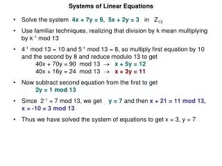
2. Simple system Solution

3. Not so simple system Solve Solution

4. Linear equations

5. Examples

6. Example

7. Linear systems

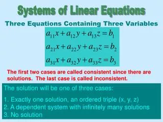
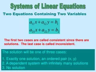
8. Consistency A system of equations that has no solution is said to be inconsistent; if there is at least one solution of the system, it is said to be consistent.

9. Solution possibilities for two lines

10. A ‘deep’ statement Every system of linear equations has either no solutions, exactly one solution, or infinitely many solutions.

11. Augmented matrices This is called the augmented matrix for the system.

12. Example Do handout Q1-Q8

13. Solving a system The main idea here is to replace the given system by a new system that has the same solution set but which is easier to solve. We apply the following three types of operations to eliminate unknowns systematically: 1. Multiply an equation by a non-zero constant. 2. Interchange two equations. 3. Add a multiple of one equation to another. These operations correspond to the following elementary row operations on the augmented matrix: 1. Multiply a row by a non-zero constant. 2. Interchange two rows. 3. Add a multiple of one row to another row.

14. An example

15. An example

16. An example

18. Echelon form We wish to reduce our matrices to those with the following properties: 1. If a row does not consist entirely of zeros, then the first nonzero number in the row is a 1. (This is called a leading 1.) 2. If there are any rows that consist entirely of zeros, then they are grouped together at the bottom of the matrix. 3. In any two successive rows that do not consist entirely of zeros, the leading 1 in the lower rows occurs farther to the right than the leading row in the higher row. 4. Each column with a leading 1 has zeros everywhere else.

19. Echelon form Echelon matrices 1. If a row does not consist entirely of zeros, then the first nonzero number in the row is a 1. (This is called a leading 1.) 2. If there are any rows that consist entirely of zeros, then they are grouped together at the bottom of the matrix. 3. In any two successive rows that do not consist entirely of zeros, the leading 1 in the lower rows occurs farther to the right than the leading row in the higher row. 4. Each column with a leading 1 has zeros everywhere else. A matrix having properties 1, 2 and 3 (but not necessarily 4) is said to be in row-echelon form. A matrix having properties 1, 2, 3 and 4 is said to be in reduced row-echelon form.

20. Reduced versus non-reduced

21. From echelon form to solution(Example 1: unique solution)

22. From echelon form to solution(Example 2: infinite solutions)

23. From echelon form to solution(Example 3: no solutions)

24. Gaussian elimination: an example

25. Gaussian elimination: an example The matrix is now in row-echelon form!

26. Gaussian elimination: an example The matrix is now in reduced row-echelon form! The above procedure for reducing a matrix to reduced row-echelon form is calledGauss-Jordan elimination. If we use only the first five steps, the procedure produces a row-echelon form and is called Gaussian elimination.

27. Not so simple system Augmented matrix Solution Row-echelon form Reduced row-echelon form

28. Back-substitution Row-echelon form Solving for the lead variables:

29. Homogeneous linear systems So a homogenous system either has only the trivial solution, or infinitely many solutions in addition to the trivial solution. All such systems are consistent.

30. Homogeneous linear systems Do Handout Q1-Q26 Theorem: A homogeneous system of linear equations with more unknowns than equations has infinitely many solutions. Note: A consistent nonhomogeneous system with more unknowns than equations also has infinitely many solutions.