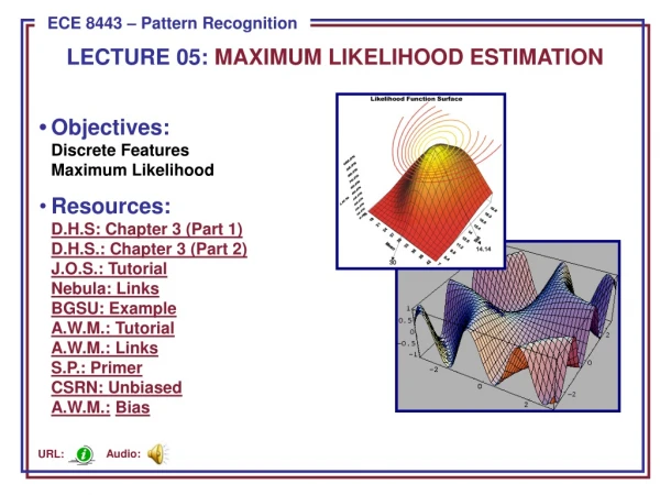
Applied Econometrics Maximum Likelihood Estimation and Discrete choice Modelling

1. Applied EconometricsMaximum Likelihood Estimation and Discrete choice Modelling Nguyen Ngoc Anh Nguyen Ha Trang

2. Content • Basic introduction to principle of Maximum Likelihood Estimation • Binary choice • RUM • Extending the binary choice • Mutinomial • Ordinal

3. Maximum Likelihood Estimation • Back to square ONE • Population model: Y = α + βX + ε • Assume that the true slope is positive, so β > 0 • Sample model: Y = a + bX + e • Least squares (LS) estimator of β: bLS= (X′X)–1X′Y = Cov(X,Y) / Var(X) • Key assumptions • E(|x) = E( ) = 0  Cov(x, ) = E(x ) = 0 • Adding: Error Normality Assumption – e is idd with normal distribution

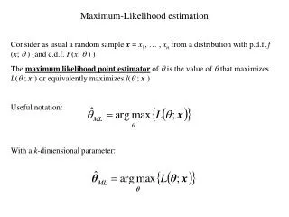
4. Maximum Likelihood Estimation • joint estimation of all the unknown parameters of a statistical model. •  that the model in question be completely specified. •  Complete specification of the model includes specifying the specific form of the probability distribution of the model's random variables. •  joint estimation of the regression coefficient vector βand the scalar error variance σ2.

5. Maximum Likelihood Estimation • Step 1: Formulation of the sample likelihood function • Step 2: Maximization of the sample likelihood function with respect to the unknown parameters β and σ2 .

6. Maximum Likelihood Estimation • Step 1 • Normal Distribution Function: if Then we have the density function From our assumption with e or u

7. Maximum Likelihood Estimation • Substitute for Y: • By random sampling, we have N independent observations, each with a pdf • joint pdf of all N sample values of Yican be written as

8. Maximum Likelihood Estimation • Substitute for Y

9. Maximum Likelihood Estimation • the joint pdf f(y) is the sample likelihood function for the sample of N independent observations • The key difference between the joint pdf and the sample likelihood function is their interpretation, not their form.

10. Maximum Likelihood Estimation • The joint pdf is interpreted as a function of the observable random variables for given values of the parameters and • The sample likelihood function is interpreted as a function of the parameters β and σ2for given values of the observable variables

11. Maximum Likelihood Estimation • STEP 2: Maximization of the Sample likelihood Function • Equivalence of maximizing the likelihood and log-likelihood functions : Because the natural logarithm is a positive monotonic transformation, the values of β and σthat maximize the likelihood function are the same as those that maximize the log-likelihood function • take the natural logarithm of the sample likelihood function to obtain the sample log-likelihood function.

12. Maximum Likelihood Estimation • Differentiation and prove that • MLE estimates is the same as OLS

13. Maximum Likelihood Estimation Statistical Properties of the ML Parameter Estimators • Consistency • 2. Asymptotic efficiency 3. Asymptotic normality Shares the small sample properties of the OLS coefficient estimator

14. Binary Response Models: Linear Probability Model, Logit, and Probit • Many economic phenomena of interest, however, concern variables that are not continuous or perhaps not even quantitative • What characteristics (e.g. parental) affect the likelihood that an individual obtains a higher degree? • What determines labour force participation (employed vs not employed)? • What factors drive the incidence of civil war?

15. Binary Response Models • Consider the linear regression model • Quantity of interest

16. Binary Response Models • the change in the probability that Yi = 1 associated with a one-unit increase in Xj, holding constant the values of all other explanatory variables

17. Binary Response Models

18. Binary Response Models • Two Major limitation of OLS Estimation of BDV Models • Predictions outside the unit interval [0, 1] • The error terms ui are heteroskedastic – i.e., have nonconstant variances.

19. Binary Response Models: Logit - Probit • Link function approach

20. Binary Response Models • Latent variable approach • The problem is that we do not observe y*i. Instead, we observe the binary variable

21. Binary Response Models

22. Binary Response Models • Random utility model

23. Binary Response Models • Maximum Likelihood estimation • Measuring the Goodness of Fit

24. Binary Response Models • Interpreting the results: Marginal effects • In a binary outcome model, a given marginal effect is the ceteris paribus effect of changing one individual characteristic upon an individual’s probability of ‘success’.

25. STATA Example • Logitprobit.dta • Logitprobit description • STATA command • Probit/logitinlfnwifeinced exp expsq age kidslt6 kidsge6 • dprobitinlfnwifeinced exp expsq age kidslt6 kidsge6