Download
1 / 25
250 likes | 364 Views
Testing the Shear Ratio Test: (More) Cosmology from Lensing in the COSMOS Field. James Taylor University of Waterloo (Waterloo, Ontario, Canada). DUEL Edinburgh,

E N D
Testing the Shear Ratio Test: (More) Cosmology from Lensing in the COSMOS Field James Taylor University of Waterloo (Waterloo, Ontario, Canada) DUEL Edinburgh, Summer Conference July 18-23 2010
The COSMOS Survey • 2 square degree ACS mosaic • lensing results from 1.64 square degrees (~600 pointings) • 2-3 million galaxies down to F814WAB = 26.6 (0.6M to 26) • 30-band photometry, photo-zs with dz ~ 0.012(1+z) to z = 1.25 and IF814W = 24 • follow-up in X-ray, radio, IR, UV, Sub-mm, …
WL Convergence Maps(cf. Rhodes et al. 2007; Massey et al. 2007; Leauthaud et al 2007) • cut catalogue down to 40 galaxies/arcmin2 to remove bad zs • correct for PSF variations, CTE • Get lensing maps, low-resolution 3D maps, various measures of power in 2D and restricted 3D • results compare well with baryonic distributions (e.g. galaxy distribution)
The Final Result: E-modes (left) versus B-modes (right)
The Final Result: 3-D constraints on the amplitude of fluctuations: recent updates: - improved photo-zs - improved CTE correction in images - new shear calibration underway + updated group catalog(s) so expect stronger signal around peaks in lensing map, and cleaner dependence on source and lens redshift time for some 2nd generation tests of the lensing signal Massey et al 2007
Measuring Geometry: Shear Ratio Test (Jain & Taylor 2003, Bernstein & Jain 2004, Taylor et al. 2007) Take ratio of shear of objects behind a particular cluster, as a function of redshift Details of mass distribution & overall calibration cancel clean geometric test Can extend this to continuous result by fitting to all redshifts Z(z) DLS/DS Relative Lensing Strength Z(z) Your cluster goes here Bartelmann & Schneider 1999
But how big is the signal? Base: h = 0.73, m = 0.27 ( or X = 1 - m) Variants (different curves): m = 0.25,0.30,0.32 w0 = -1,-0.95,-0.9,-0.85,-0.8 w(z) = w0 + wa(1-a) with w0 = -1, wa = 0.05, 0.1 h = 0.7, 0.75 Use strength of signal behind cluster as a function of redshift to measure DA(z):
How big is the signal? Base: h = 0.73, m = 0.27 ( or X = 1 - m) Variants (different curves): m = 0.25,0.30,0.32 w0 = -1,-0.95,-0.9,-0.85,-0.8 w(z) = w0 + wa(1-a) with w0 = -1, wa = 0.05, 0.1 h = 0.7, 0.75 Lens at z = 0.2 Use strength of signal behind cluster as a function of redshift to measure DA(z): weak but distinctive signal; relativechange (change in distance ratio)is only 0.5% 0.5% relative change
How big is the signal? Base: h = 0.73, m = 0.27 ( or X = 1 - m) Variants (different curves): m = 0.25,0.30,0.32 w0 = -1,-0.95,-0.9,-0.85,-0.8 w(z) = w0 + wa(1-a) with w0 = -1, wa = 0.05, 0.1 h = 0.7, 0.75 Lens at z = 0.3 Use strength of signal behind cluster as a function of redshift to measure DA(z): weak but distinctive signal; relativechange (change in distance ratio)is only 0.5% 0.5% relative change
How big is the signal? Base: h = 0.73, m = 0.27 ( or X = 1 - m) Variants (different curves): m = 0.25,0.30,0.32 w0 = -1,-0.95,-0.9,-0.85,-0.8 w(z) = w0 + wa(1-a) with w0 = -1, wa = 0.05, 0.1 h = 0.7, 0.75 Lens at z = 0.5 Use strength of signal behind cluster as a function of redshift to measure DA(z): weak but distinctive signal; relativechange (change in distance ratio)is only 0.5% 0.5% relative change
How big is the signal? Base: h = 0.73, m = 0.27 ( or X = 1 - m) Variants (different curves): m = 0.25,0.30,0.32 w0 = -1,-0.95,-0.9,-0.85,-0.8 w(z) = w0 + wa(1-a) with w0 = -1, wa = 0.05, 0.1 h = 0.7, 0.75 Lens at z = 0.7 Use strength of signal behind cluster as a function of redshift to measure DA(z): weak but distinctive signal; relativechange (change in distance ratio)is only 0.5% 0.5% relative change
How big is the signal? Base: h = 0.73, m = 0.27 ( or X = 1 - m) Variants (different curves): m = 0.25,0.30,0.32 w0 = -1,-0.95,-0.9,-0.85,-0.8 w(z) = w0 + wa(1-a) with w0 = -1, wa = 0.05, 0.1 h = 0.7, 0.75 Signal weak but distinctive Lens at z = 1.0 Use strength of signal behind cluster as a function of redshift to measure DA(z): weak but distinctive signal; relativechange (change in distance ratio)is only 0.5% 0.5% relative change
Previous detections with massive clusters Signal has been seen previously behind a few clusters: e.g. Wittman et al. 2001 ~3e14 Mo cluster in DLS; detection, mass and redshift all from weak lensing (source photo-zs from 4 bands)
Previous detections with massive clusters Signal has been seen previously behind a few clusters: e.g. Gavazzi & Soucail (2008): cluster Cl-02 in CFHTLS-Deep (cf. also Medezinski et al. submitted: 1.25 M galaxies behind 25 massive clusters, in a few bands)
So why try this in COSMOS ? Less signal (groups only, no truly massive clusters), but far better photo-zs can push techniques down to group or galaxy scales nice test of systematics in catalogue selection, effect of photo-z errors test/confirm error forecasts for future surveys Percival et al .2007: interesting indication of possible mismatch in distance scales in BAO?
The sample of COSMOS Groups and Clusters (X-ray derived Mass) Log(volume) (plot from Leauthaud et al. 2009)
~67 in top 14 objects? The sample of COSMOS Groups and Clusters (X-ray derived Mass) Log(volume) (plot from Leauthaud et al. 2009)
could get another ~60 from less massive groups? The sample of COSMOS Groups and Clusters (X-ray derived Mass) Log(volume) (plot from Leauthaud et al. 2009)
Shear vs. photo-z around peaks, along promising lines of sight
Shear vs. photo-z around peaks, along promising lines of sight
How to stack clusters? Tangential shear goes as: so redshift dependence enters via critical surface density: Thus if we define (assumes flat models) and then independent of cosmology
We see the signal! Stack of regions within 6’ of ~200+ x-ray groups good fit in front of/behind cluster significance still unclear; seems less than expected effect of other structures along the line of sight decreases chi2, but hard to quantify
A Caveat In a field this small, a few redshifts dominate the distribution of structure systematics in shear ratio
Signal detected, well behaved, significance slightly lower than expected? • Still studying noise versus radial weighting, catalogue cuts, path weighting • Results roughly consistent with w0 ~ -1.0 +/- 1.0 • Future predictions for large surveys + CMB + BAO (Taylor et al. 2007): • w0 = 0.047, wa = 0.111 and 2% • measurement of dark energy at • z ~ 0.6 • Or use CMB as an extra slice? • (cf. Hu, Holz & Vale 2007; • Das & Spergel 2009) Prospects error forecasts from 20,000 deg2 survey (Taylor et al. 2007)