Download
1 / 64
640 likes | 839 Views
COS 131: Computing for Engineers Ch. 3: Vectors and Arrays. Laura Broussard, Ph.D. Professor. Ch. 3: Vectors and Arrays. Introduction Concept: Using Built-in Functions Concept: Data Collections MATLAB Vectors Engineering Example MATLAB Arrays Engineering Example.

E N D
COS 131: Computing for EngineersCh. 3: Vectors and Arrays Laura Broussard, Ph.D. Professor
Ch. 3: Vectors and Arrays • Introduction • Concept: Using Built-in Functions • Concept: Data Collections • MATLAB Vectors • Engineering Example • MATLAB Arrays • Engineering Example
I. Introduction • Emphasizes the basic calculations involving rectangular collections of numbers in the form of vectors and arrays. • You will learn how to: • Create them • Manipulate them • Access them • Perform mathematical/logical operations on them • Shows MATLAB’s ability to deal with sets of numbers as aggregates as opposed to individually • Introduces the notion of functions built into the language
Ch. 3: Vectors and Arrays • Introduction • Concept: Using Built-in Functions • Concept: Data Collections • MATLAB Vectors • Engineering Example • MATLAB Arrays • Engineering Example
II. Concept: Using Built-in Functions • Function – a named collection of instructions that operates on the data provided to produce a result according to the specifications of that function • To get help on a particular function, type the following at the Command window prompt: • >> help <function name>
III. Concept: Data Collections • MATLAB groups data together in arrays and in vectors (subsets of arrays) • Data Abstraction • Convenient to refer to groups of data as opposed to individual data items • Allows the movement of these data as a group • Allows the use of mathematical and/or logical operations on these groups
III. Concept: Data Collections • Homogeneous Collection • Arrays and vectors constrain data to only be accepted for the same data type • These are referred to as homogeneous collections; i.e., all data items within a given array or vector are of the same data type • We will now consider the basic operations related to vectors and arrays in MATLAB
Ch. 3: Vectors and Arrays • Introduction • Concept: Using Built-in Functions • Concept: Data Collections • MATLAB Vectors • Engineering Example • MATLAB Arrays • Engineering Example
IV. MATLAB Vectors • Vector – a list of like data items (simplest means of grouping) • Elements – individual items in a vector • Elements have two attributes: • Numerical value • Position in the given vector • Data type: numbers or logical values • Vectors also called linear arrays or linear matrices
IV. MATLAB Vectors • Creating Vectors • Size (measuring) • Indexing • Shortening • Operations Arithmetic Concatenation Logical Slicing Library
IV. MATLAB Vectors • Creating Vectors – 2 methods • Creating vectors as a series of constant values • Producing new vectors by operating on existing vectors (later)
IV. MATLAB Vectors A. Creating Vectors - from constant values: • Enter each value directly A = [1 2 3] • Enter a range of values with colon operator B = 1:3:20 • Entering a range of values with linspace(…) function C = linspace (0, 20, 11)
IV. MATLAB Vectors • Creating from constant values (cont’d.) • Using functions: zeros(1,n) rand(1,n) ones(1,n) randn(1,n) for vectors with 0’s, 1’s, or random numbers in between E = zeros(1,4) Exercise 3.1 Working with Vectors, pp. 49-50
IV. MATLAB Vectors • Creating vectors • Workspace window information • The name • The value Contents (small vectors) or Description - such as <1 x 11 double> • The class (data type) of the vector • Scalars are vectors (unit length)
IV. MATLAB Vectors • Size of a Vector • Specific attribute – the length of the vector; how many elements are in the vector • Can increase or decrease the size of a vector by inserting and deleting elements • Function size(V) when applied to vector V, returns another vector [r, c]: r = number of rows (for vectors, 1) c = number of columns (length of vector) • Function length(V) returns the length of the vector
IV. MATLAB Vectors • Indexing a Vector • Definition: accessing elements of a vector to assess its value and/or change the value • Two ways of indexing: • With a numerical vector • With a logical vector • Numerical indexing • Elements of a vector can be accessed individually or in groups by enclosing the index of one or more required elements in parentheses
IV. MATLAB Vectors • Indexing a Vector • Numerical Indexing: A = [0 2 4 68] • Assessing value: >> A(1) ans = 0 • Changing value: >> A(1) = 6 A = [6 2 4 68] Exercise 3.2, Extending a vector, p. 51b • MATLAB will automatically extend a vector if you write beyond its current end. Missing elements zero-filled Exercise 3.3, Extending a vector, p. 51b • These examples use a single number to index
IV. MATLAB Vectors • Indexing a Vector • Numerical Indexing A = [0 2 4 6 8] • Indexing can also be with multiple numbers. >> A(1),(2),(3) ans = 0 ans = 2 ans = 4 • Use a vector of index values to index another vector >> B = [ 1 3 5 ] >> A(B) ans = 0 4 8 (Note: argument of A is a vector) • Index vector: - doesn’t need to match size of vector being indexed - values must be positive and smaller than length of vector being indexed
IV. MATLAB Vectors • Indexing a Vector • Logical Indexing A = [0 2 4 6 8] • A new (for us) data type. • Two values: true and false • Called Boolean or logical values • Can be assembled into vectors and arrays by typing in true or false values. MATLAB responds with 0’s and 1’s >> mask = [true false false true] mask = 1 0 0 1 >> A(mask) ans = 0 6 • Logical index vectors can be shorter, not longer.
IV. MATLAB Vectors • Shortening a Vector A = [0 2 4 6 8] • May need to remove elements from a vector • Use the empty vector, [ ] A vector with no elements in it • Assign the empty vector to an element in another vector, that element is removed from A, and A is shortened by on element >> A(4) = [ ] A = [0 2 6 8] • Exercise 3.4: Shortening a vector, p. 52b
IV. MATLAB Vectors • Operating on Vectors • Three techniques analogous to operations on scalar (single) values: • Arithmetic operations • Logical operations • Applying library functions • Two unique techniques for vectors and arrays: • Concatenation (joining) • Slicing (generalized indexing)
IV. MATLAB Vectors • Operations - Arithmetic • Can be performed collectively on individual components of two vectors if • both vectors are same length or • one of the vectors is scalar (one value) • Element by element NOT matrix operations • Use symbols: .*, ./, and .^ Regular symbols *, /, and ^ reserved for matrix operations.
IV. MATLAB Vectors • Operations – Arithmetic • Addition and subtraction same for both matrix and element-by-element operations Use the same symbols: + and - • Exercise 3.5: Using vector mathematics, pp. 53-54
IV. MATLAB Vectors • Logical Operations • Produce vectors of logical results • Use to index vectors in a style that makes the logic of complex expressions very clear • Can perform element-by-element operations on two vectors if both vectors are the same length or if one is a scalar • A = [2 5 7 1 3] and B = [0 6 5 3 2] • Where are A’s elements ≥ 5? • >> A >= 5 ans = 0 1 1 0 0 • >> A >= B ans = 1 0 1 0 1 • Ex 3.6, Working with vector logical expressions, p. 55t
IV. MATLAB Vectors • Logical Operations • Can be assembled into more complex operations using logical and (&) and or (|) operators • Operators come in two flavors • & / | (single operators) • && / || (double operators) • Single operators are for logical arrays of matching size • Double operators combine individual logical results, and are associated with conditional statements (Ch. 7) • Exercise 3.7, Working with logical vectors, p. 55b
IV. MATLAB Vectors • Logical Operations • Function find(…) Inputs an array of logical values Outputs a vector of positions of true elements Useful to find indices of the true elements of a logical vector • Ex. 3.8: Using the find(…) function, p. 56 t
IV. MATLAB Vectors • Logical Operations a = [true true false true ] • Negate the values of all elements of a logical vector (true ⇒ false and false ⇒ true) with ~ (not operator) >> na = ~[true true false true] na = 0 0 1 0 • Each element of na is the logical inverse of the corresponding original element • Table 3.1, Operator Precedence, p. 56
IV. MATLAB Vectors • Operations - Library Functions • MATLAB has a rich collection of mathematical functions covering mathematical, trigonometric, and statistical capabilities • Partial list in App. A • Complete list – Help menu option • Accept vectors of numbers rather than single values and return a vector of the same length
IV. MATLAB Vectors • Operations - Useful Library Functions • sum(v) and mean(v) consume a vector and return the sum and mean of all the elements of the vector • min(v) and max(v) return two quantities: the minimum and maximum value in vector the position of the value in vector >> [value where] = max([2 7 42 9 -4]) value = 42 where = 2 • round(v), ceil(v), floor(v), and fix(v) functions that round numbers in vector
IV. MATLAB Vectors • Operations - Concatenation • MATLAB lets you construct a new vector by concatenating (joining) other vectors • A = [B C D … X Y Z] B, C, D, … are any vector sdefined as a constant or variable length of A is sum of the lengths of B, C, D, … • Resulting vector will be flat, not nested. • Exercise 3.9: Concatenating Vectors, p. 57b
IV. MATLAB Vectors • Operations: Slicing • Indexing ≡ basic operation of extracting and replacing the elements of a vector – Vectors of indices ⇒ change multiple elements – Vectors can be: ⋄ previously-defined indices or ⋄ created anonymously as needed
IV. MATLAB Vectors • Operations: Slicing – Anonymous A = [2 5 7 1 3 4] • General form for generating a vector of numbers: <start> : < increment> : <end> Omit <increment>, default = 1 Key word end ≡ the length of the vector Operator : (alone) is short for 1:end odds = 1:2:end • Indexing vector of logical values must be same length or shorter than the vector being indexed >> A([false true false true]) ans = 5 1
IV. MATLAB Vectors • Operations - Slicing • General form of statements for slicing vectors (copy part of A to part of B) B(<rangeB> = A(<rangeA>) • When <rangeA> and <rangeB> are index vectors, • A is an existing Array • B can be an existing or new array or absent altogether (named ans) • Rules on next slide
IV. MATLAB Vectors • Operations - Slicing • Rules for use of this template: • Either - size of rangeB = size of rangeA or - size of rangeA = 1 • If B does not exist, it is zero-filled where assignments not explicitly made • If B did not exist before this statement, values of A not directly assigned in rangeB remain unchanged • See Listing 3.1 on the next slide
IV. MATLAB Vectors • Slicing
IV. MATLAB Vectors • Operations – Slicing • Ex 3.10 Running the vector indexing script, pp. 59-60 • Refer to line by line description on page 59-61. This will become commonplace in our class discussions as we examine MATLAB code to understand what the software is doing.
Ch. 3: Vectors and Arrays • Introduction • Concept: Using Built-in Functions • Concept: Data Collections • MATLAB Vectors • Engineering Example • MATLAB Arrays • Engineering Example
V. Engineering Example – Forces and Moments • MATLAB vectors are ideal representations of the concept of a vector used in physics • Represent each of the vectors in this problem as a MATLAB vector with three components: the x, y, and z values of the vector
V. Engineering Example – Forces and Moments Examine code to left and work through commentary on page 64.
Ch. 3: Vectors and Arrays • Introduction • Concept: Using Built-in Functions • Concept: Data Collections • MATLAB Vectors • Engineering Example • MATLAB Arrays • Engineering Example
VI. MATLAB Arrays • We now extend the vector ideas to include arrays of multiple dimensions • Initially two dimensions • Each row will have the same number of columns and each column will have the same number of rows • Referred to as arrays to differentiate them from matrices • Arrays and matrices differ in the way they execute their multiplication, division, and exponentiation operations
IV. MATLAB Arrays • Properties • Creating • Accessing Elements • Removing Elements • Operations Arithmetic Concatenation Logical Slicing Library Reshaping Linearizing
MATLAB Arrays • Properties of an Array • Individual elements in an array are also referred to as elements • Unique attributes: value and position • In a 2-D array position will be (row, column) • In an n-D array, the element position will be a vector of n index values
MATLAB Arrays • Properties of an Array • Function size will return information 1 of 2 forms: • If called with a single return value sz = size(A) It returns a vector of length n containing the size of each dimension of the array • If called with multiple return values [rows, cols] = size(A) It returns the individual array dimension up to the number of values requested; ALWAYS provide as many variables as there are dimensions of the array
MATLAB Arrays • Properties of an Array • The length(…) function returns the maximum dimension of the array • The transpose of an m x n array, indicated by the apostrophe character (‘) placed after the array identifier, returns an n x m array with the values in the rows and columns interchanged. • See example on the next slide
MATLAB Arrays • Properties of an Array Original Array Transposed Array
MATLAB Arrays • Properties of an Array • Special Cases: • When a 2-D matrix has the same number of rows and columns, it is called square • When only nonzero values in an array occur when the row and column indices are the same, the array is called diagonal • When there is only one row, the array is a row vector, or just a vector as we saw earlier • When there is only one column, the array is a column vector, the transpose of row vector
MATLAB Arrays • Creating an Array • Created by entering values directly • Created by using one of a number of built-in MATLAB functions that create arrays with specific characteristics: • Enter data directly, using a ; to denote the end of a row • Functions zeros(m,n) and ones(m,n) creates an m x n matrix with zeros or ones • Functions rand(m,n) and randn(m,n) fill an array with random numbers in the range 0 .. 1. • Function diag(…) where diag(A) of an array A returns its diagonal as a vector, and diag(V) of a vector returns a square array with the vector as the diagonal • Function magic(m) which produces an m x m array which returns a square array where the values in rows and columns add up to the same value
MATLAB Arrays • Creating an Array • Exercise 3.11: Creating Arrays • Smith text, page 67, top
MATLAB Arrays • Accessing Elements of an Array • Elements of an array may be addressed by enclosing the indices of the required elements in parentheses, with the first index being the row index and the second index the column index • Can also store values that are elements of an array as in A(2,3) = 0 will assign the value of 0 to the cell that is at row 2, column 3. • MATLAB automatically extends the array if you write beyond its boundaries. Elements with no values between the boundaries of the array will be assigned values of zero, 0.