Download

1 / 24
240 likes | 1.01k Views
Best-Fitting Bezier Curves for Graphs of Functions. Outline. This presentation looks at finding optimal Bezier curves Background and definitions Eight unknowns: Six constraints based on the functions and derivatives Two constraints based on minimizing the mean squared error

E N D
Outline • This presentation looks at finding optimal Bezier curves • Background and definitions • Eight unknowns: • Six constraints based on the functions and derivatives • Two constraints based on minimizing the mean squared error • Ten examples of various functions
Background Bezier curves are used to model smooth space curves Often necessary to plot specific functions, including: Circles Exponential Trigonometric functions We will define a technique for finding such curves and look at some examples
Mathematical Notation We will use standard mathematical notation to represent various values: Variables are italicized lower-case characters t, x, y, a, b Vectors are bold lower-case characters vk Functions are roman lower-case characters f(t), x(t), y(t) Derivatives are represented as superscripts f(1)(t)
Theory Given a vector space, a cubic Bezier curve is defined by four vectors v1, v2, v3, v4 and uses these to define a space curve parametrically v1(1 – t)3 + v2t(1 – t)2 + v3t2(1 – t) + v4t3 with t varying from 0 to 1 We will use vk = (xk, yk)
Theory To find the best fitting Bezier curve for the graph of a function (x, f(x)) for x on an interval [a, b], introduce three constraints: v1 = (a, f(a)) v4 = (b, f(b)) We will also require that the derivatives match: f(1)(a) = (y2 – y1)/(x2 – x1) f(1)(b) = (y4 – y3)/(x4 – x3) where vk = (xk, yk)T
Theory To deal with functions which have asymptotes in the derivative, to constrain the size, we will make one of two substitutions: If |f(1)(a)| < 1, substitute y2 = f(a) + f(1)(a) (x2 – a), else substitute x2 = (y2 – f(a))/f(1)(a) + a Similarly, if |f(1)(b)| < 1, substitute y3 = f(b) + f(1)(b) (x3 – b), else substitute x3 = (y3 – f(b))/f(1)(b) + b
Theory With these substitutions, we now have two Bezier curves with two unknown variables These define the Bezier curve parametrically There are four cases for the substitutions: If both derivatives are small, the two curves are x(t) = a(1 – t)3 + x2t(1 – t)2 + x3t2(1 – t) + bt3 y(t) = f(a)(1 – t)3 + [f(a) + f(1)(a) (x2 – a)]t(1 – t)2 + [f(b) + f(1)(b) (x3 – b)]t2(1 – t) + f(b)t3 If the derivative is large (or infinity) at the left point, use: x(t) = a(1 – t)3 + [(y2 – f(a))/f(1)(a) + a]t(1 – t)2 +x3t2(1 – t) + bt3 y(t) = f(a)(1 – t)3 +y2t(1 – t)2 + [f(b) + f(1)(b) (x3 – b)]t2(1 – t) + f(b)t3
Theory We must now define a function which must be minimized We will minimize the root mean-squared error: This is a real-valued bivariate function in the two unknown parameters Use techniques such as gradient descent to find the minimum Reasonable initial approximations are the midpoints: xk = (a + b)/2 yk = (f(a) + f(b))/2
Theory Why minimize the root mean squared error? The error is a continuous and differentiable function in the parameters Squaring emphasizes larger errors relative to smaller errors One could also minimize the infinity norm: Continuous, but not differentiable
Examples The following ten slides gives the best fitting Bezier curves for a number of functions on specific intervals The function is plotted in red The best fitting Bezier curve is plotted in blue behind the graph of the function The code was written in the Maple programming language The source code is available at http://ece.uwaterloo.ca/~dwharder/Maplesque/Bezier/
Examples The best fitting Bezier curve for the quarter circle is defined by the points (0, 1), (0.5520, 1), (1, 0.5520), (1, 0) with a root mean squared error of 0.000175
Examples The best fitting Bezier curve for the sin function on[0, p/2] is defined by the points (0, 0), (0.5251, 0.5251), (1.005, 1), (1.571, 1) with a root mean squared error of 0.000474
Examples The best fitting Bezier curve for the exponential function on [0, 1] is defined by the points (0, 1), (0.3765, 1.3765), (0.7057, 1.9184), (1, 2.7183) with a root mean squared error of 0.00000102
Examples The best fitting Bezier curve for the natural logarithm function on [1, 2] is defined by the points (0.5, -0.6931), (0.8043, -0.08448), (1.3010, 0.3437), (2, 0.6931) with a root mean squared error of 0.000238
Examples The best fitting Bezier curve for the quadratic function on[0, 1] is defined by the points (0, 0), (0.4174, 0), (0.7629, 0.5257), (1, 1) with a root mean squared error of 0.000118
Examples The best fitting Bezier curve for the square root function (quadratic inverse) on [0, 1] is defined by the points (0, 0), (0, 0.4182), (0.5274, 0.7637), (1, 1) with a root mean squared error of 0.000124
Examples The best fitting Bezier curve for the function f(x) = x3/2 on[0, 1] is defined by the points (0, 0), (0.1804, 0), (0.5792, 0.3689), (1,1) with a root mean squared error of 0.00251
Examples The best fitting Bezier curve for the function f(x) = x ln(x) on [1, 10] is defined by the points (1, 0), (3.0993, 2.0993), (6.5721, 11.7052), (10., 23.0259) with a root mean squared error of 0.0202
Examples The best fitting Bezier curve for the standard normal curve on [0, 3] is defined by the points (0,1), (0.9235, 1), (0.1722, 0.002217), (3, 0.0001234) with a root mean squared error of 0.0490
Examples It is better to use two Bezier curves on [0, 1] and [1, 3]: (0, 0.5642), (0.3452, 0.5642), (0.6314, 0.3605), (1, 0.2076) (1, 0.2076), (1.5128, -0.005325), (1.8960, 0.0005308), (3, 0.00006963) with a root mean squared errors of 0.0000147 and 0.000227
Examples The best fitting Bezier curve for the sinc function (sin(x)/x or the cardinal sine) on [0, p] is defined by the points (0,1), (1.1339, 1), (2.0493, 0.3477), (3.1416, 0) with a root mean squared error of 0.000154
Summary • This presentation looked at finding optimal Bezier curves for function graphs: • Six constraints are defined by the properties of the graph • Two are found by minimizing the root mean squared error • The results are usually very good • The function x1.5 resulted in the worst case • The smooth exponential function was best fit
Usage Notes • These slides are made publicly available on the web for anyone to use • If you choose to use them, or a part thereof, for a course at another institution, I ask only three things: • that you inform me that you are using the slides, • that you acknowledge my work, and • that you alert me of any mistakes which I made or changes which you make, and allow me the option of incorporating such changes (with an acknowledgment) in my set of slides Sincerely, Douglas Wilhelm Harder, MMath dwharder@alumni.uwaterloo.ca