Aggregate Expenditure
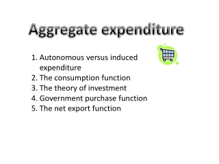
Aggregate Expenditure. Outline Components of aggregate expenditure Planned and unplanned expenditure The consumption function Imports and GDP Equilibrium expenditure The expenditure multiplier. Components of Aggregate Expenditure.

Aggregate Expenditure
E N D
Presentation Transcript
Aggregate Expenditure • Outline • Components of aggregate expenditure • Planned and unplanned expenditure • The consumption function • Imports and GDP • Equilibrium expenditure • The expenditure multiplier
Components of Aggregate Expenditure • Recall from Chapter 5 that aggregate expenditure for final goods and services equals the sum of • Consumption expenditure, C • Investment, I • Government purchases of goods and services, G • Net exports, NX Thus:Aggregate expenditure = C + I + G + NX
Planned and Unplanned Expenditures Aggregate expenditure aggregate income and real GDP. But aggregate planned expenditure might not equal real GDP because firms can end up with larger or smaller inventories than they had intended.
Autonomous versus induced Expenditure • Autonomous expenditure: The components of aggregate expenditure that do not change when real GDP changes. • Induced expenditure: The components of aggregate expenditure that change when real GDP changes.
The Consumption Function The consumption function shows the relationship between consumption expenditure and disposable income, holding all other influences on influences on household spending behavior constant.
What is disposable income? • Disposable income is aggregate income (GDP) minus net taxes • Net taxes are taxes paid to government minus transfer payments received from government.
www.bea.gov 1991
450 line Consumption (trillions of 1996 dollars) Saving F Consumption function E D 6.0 Dissaving C Saving is zero B 2.0 A 2.0 6.0 10.0 Disposable income (trillions of 1996 dollars) (trillions of 1996 dollars)
Notice that autonomous consumption is given by point A. This is planned consumption expenditure when disposable income is zero ($1.5 trillion). This spending must be financed by past saving or by borrowing
Marginal Propensity to Consume (MPC) The marginal propensity to consume (MPC) is the fraction of the change in disposable income that is spent on consumption. That is: Change in consumption expenditure MPC = Change in disposable income Notice that when disposable income increases from $6 to $8 trillion, consumption expenditure changes from $6.0 to $7.5 trillion. Thus we have:
MPC gives the slope of the consumption function Consumption function E 7.5 D rise Consumption (trillions of 1996 dollars) 6.0 K run 0 6.0 8.0 Disposable income (trillions of 1996 dollars)
Determinants of Consumption Expenditure Disposable income + (Expected) real interest rate - RealConsumptionSpending + The buying power of net assets + Expected future disposable income
Shifts of the consumption function • CF0 to CF1 • Decrease in the real interest rate. • Buying power of net assets increases. • Rise in expected future disposable income. CF1 CF0 CF2 Consumption (trillions of 1996 dollars) 0 Disposable income (trillions of 1996 dollars)
Falling interest rates have stimulated consumer spending recently
Imports and GDP Imports are a component of induced expenditure. Imports depend partly on the health of the domestic economy.
Marginal Propensity to import (MPI) The marginal propensity to import (MPI) is the fraction of the change in disposable income that is spent on imports . That is: Change imports MPI = Change in disposable income Suppose that, ceteris paribus, when disposable income increases from $2 trillion, imports increase by $0.3 trillion. Thus we have:
Aggregate Expenditure and Real GDP Note: Y is real GDP
I + G + C + X Agg. Exp. (billions of 1996 dollars) imports AE D Consumption expenditure C I + G + X 4.5 A 3 I + G I 0 9 GDP (Billions of 1996 dollars)
AE (trillions of 1996 dollars) AE J 12 F D 9 B 6 K 450 0 3 9 15 GDP (trillions of 1996 dollars)
Case 1: GDP = $3 trillion • AE > GDP by vertical distance B-K • Plans of producing and spending units do not coincide • Unplanned inventory investment = - $3 trillion • Tendency for firms (on average) to step up the pace of production and offer more employment
Case 2: GDP = $15 trillion • GDP > AE by vertical distance J-F • Plans of producing and spending units do not coincide • Unplanned inventory investment =$3 trillion • Tendency for firms (on average) to scale back the on production and offer less employment
Case 3: GDP = $9 trillion • AE = GDP • Plans of producing and spending units coincide. • Unplanned inventory investment = 0 • No tendency for firms (on average) to step up the pace of production and offer more employment. Nor is there a tendency for firms to scale back on production and offer less employment.
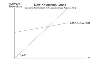
Say’s Law1 • “Supply creates its own demand.” • By producing goods and services, firms create a total demand for goods and services equal to what they have produced. Say’s law apparently rules out the possibility of a widespread glut of goods. 1 J.B. Say. Treatise on Political Economy, 1903.
Say’s law implies that full-employment equilibrium is the normal state of affairs AE C + I + G + NX AE touchesthe 450 line at potential GDP Full employment GDP GDP
General (Keynesian) Case: Underemployment Equilibrium AE A C + I + G + NX H Y* Full employment GDP GDP
What happens when things change? • Assume the economy is in equilibrium when real GDP = $3 trillon. • What would happen if, other things being equal, planned investment (I) increased by $0.5 trillion?
How did a $0.5 trillion change in Ibring about a $2 trillion change in GDP? AE2 AE 2 AE1 1 5 I 4.5 GDP 450 0 9.0 11.0 GDP
It’s a bird It’s a plane No, it’s the multiplier effect!
The expenditure multiplier The multiplier is amount by which a change in any component of autonomous expenditure is magnified or multiplied to determine the change that it generates in equilibrium expenditure and real GDP. Change in equilibrium expenditure Multiplier = Change in autonomous expenditure Thus in our case the multiplier is given by:
Chain of causation When firms increase investment by $0.5 trillion, sales revenues at investment goods manufacturers (Boeing, Westinghouse, Cincinnati Milacron) will increase by $0.5 trillion 1 The $0.5 trillion in revenue will be distributed as factor payments to those supplying resources necessary to produce capital goods—hence the change in spending generates $0.5 trillion in income in the first round. 2
Now households have $1,000 in additional income. What do they do with it? Their spending will increase by the MPC times the change in income—that is: C = .75 $0.5 trillion = $0.375 trillion Hence, households spend $375 billion and save $125billion 3 But the story does not end here, since McDonalds’s, Disney, Kraft, American Airlines, and Amheiser Busch, etc. will see their sales increase by $375 billion, and will distribute $375 billion in wages, salaries, rental income, and profits to those who supplied resources necessary to produce the additional consumer goods. 4
Those who earned additional income in consumer goods industries will now increase their spending. By how much?C = .75 $375 = $281.85. 5 This will result in additional production and factor payments. Spending will then increase. And so on. And so on. 6
Why is the multiplier greater than 1? As we see from the preceding illustration, a change in autonomous expenditure (in this case, I) induces a change in consumption expenditure.
The Multiplier and the MPC We will now illustrate why the magnitude of the multiplier depends on the MPC. For the moment, assume no imports, exports, or taxes. Thus: [1] Where: [2] Now substitute [2] into [1] to obtain: [1]
Now solve for Y [4] Now rearrange [4] [5] Divide both sides of [5] byI to obtain the multiplier The expenditure multiplier
You can see from the math that the size of the multiplier is positively linked to the MPC. The higher the MPC, the greater the “induced” expenditure resulting from a change in autonomous expenditure
Taxes, Imports, and the Multiplier Once we allow for imports and taxes, the multiplier depends not only on the MPC, but also on the marginal propensity to import (MPI) and the marginal tax rate (MTR)
Marginal Tax Rate (MTR) The marginal tax rate (MTR) is the fraction of the change in real GDP that is paid income taxes. That is: Change in tax payments MTR = Change in real GDP Suppose that, ceteris paribus, when real GDP increases by $0.5 trillion, tax payments increase by $0.05 trillion. Thus we have:
The “real” expenditure multiplier The multiplier is given by The slope of the AE curve is given by: Slope of AE curve = MPC – (MPI + MTR) Thus the multiplier can be written as:
In this case, MPC = 0.75; MPI = 0.15; MTR = 0.1 Slope = 0.5 AE2 AE 2 AE1 1 5 I 4.5 Y 450 0 9.0 10.0 GDP