Download
1 / 48
480 likes | 662 Views
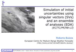
Simulation of initial uncertainties using singular vectors (SVs) and an ensemble of analyses (EDA) ( EC/TC/PR/RB-L3). Roberto Buizza European Centre for Medium-Range Weather Forecasts (http://www.ecmwf.int/staff/roberto_buizza/). Outline. The original SV-based ECMWF ensemble

E N D
Simulation of initial uncertainties using singular vectors (SVs) and an ensemble of analyses (EDA) (EC/TC/PR/RB-L3) Roberto Buizza European Centre for Medium-Range Weather Forecasts (http://www.ecmwf.int/staff/roberto_buizza/)
Outline • The original SV-based ECMWF ensemble • Ensemble Data Assimilation characteristics • The new EDA-SVINI ensemble
Definition of the perturbed ICs NH SH TR Products 1 2 50 51 ….. 1. The operational ensemble in 2013 • The operational version of the ENS includes 51 forecasts with resolution: • TL639L62 (~32km, 62 levels) from day 0 to 10 • TL319L62 (~64km, 62 levels) from day 10 to 15 (32 at 00UTC on Thursdays). • Initial uncertainties are simulated by adding to the unperturbed analyses a combination of T42L62 singular vectors, computed to optimize total energy growth over a 48h time interval (OTI), and perturbations generated using the new ECMWF Ensembles of Data Assimilation (EDA) system. • Model uncertainties are simulated by adding stochastic perturbations to the tendencies due to parameterized physical processes (SPPT scheme). • ENS is run twice a day, at 00 and 12 UTC.
1. The original ENS (before 2010) Each ensemble member evolution is given by the time integration of perturbed model equations starting from perturbed initial conditions The model tendency perturbation is defined at each grid point by where rj(t;Φ,λ) is a random number.
1. The original ENS (before 2010) The initial perturbations do not sample the tropics in an appropriate way. The system is not ‘reliable’ (spread under estimation). +48h T=0 +120h
1. std/EM of ECMWF 399v255 and 639v319 ENS NH: apart for the first 2 days the spread-skill relationship is very good, with the 639v319 version (implemented in Jan 2010) showing a better match. Tropics: both systems are under-dispersive for the whole forecast range. Is this a symptom of a weakness of the initial perturbation strategy? 399v255 (up uo Jan 2010) 639v319 399v255 (up to Jan 2010) 639v319
1. The TIGGE ensembles (updated May 2013) The 10 TIGGE ensembles use different methodologies to simulate initial-time and model uncertainties. Every day, they provide 557 global forecasts!
Outline • The original SV-based ECMWF ensemble • Ensemble Data Assimilation characteristics • The new EDA-SVINI ensemble
2. The ECMWF 4D-Var data-assimilation system The ECMWF 4-dimensional data-assimilation system determines a correction to the background initial condition (blue line) that would lead to a forecast trajectory (red line) that passes closer to the observations (red circles).
2. The assimilation problem Denote by x the atmospheric state, M(x) the (non-linear) model, xb a first-guess (background) state, H(x) the observation operator, ε.. the error fields. where the model, background and observations errors are assumed to be independent and have probability density functions Pm(εm,t), Pb(εb,t), Po(εo,t). This assumption (of independence) means that the total probability density function can be written as the product of the three: The optimal analysis xa is the state for which the total pdfP is maximum. x H(x) y y1 0 t1 time (Adapted from E. Holm, 2008: Lecture notes on assimilation algorithms, ECMWF)
2. The assimilation problem Finding the state x(0) for which the total pdfP is maximum is equivalent to finding the state x(0) for which the negative of the exponent of P has a minimum Compared to the background (blue line), following the assimilation of the observation y1 at time t1, the new forecast trajectory starting from x(0) goes closer to y1. x x H(x) H(x) y y time time y1 y1 0 0 t1 t1 (Adapted from E. Holm, 2008: Lecture notes on assimilation algorithms, ECMWF)
2. The assimilation problem Example. Suppose that the model error can be neglected (εm=0) and that the observation and model errors can be modelled by a Gaussian distribution The cost function is: The analysis state xa, is the state x that minimizes J: (Adapted from E. Holm, 2008: Lecture notes on assimilation algorithms, ECMWF)
2. The assimilation problem Now let’s approximate H(x) using its linear approximation H, and its adjointH(x)T by the adjoint of its linear approximation HT: Then the linearized equation becomes: The solution is: observation error covariance background error covariance in observation space (Adapted from E. Holm, 2008: Lecture notes on assimilation algorithms, ECMWF)
2. The ECMWF EDA Each observation has an error (instrument, representativeness) and also each model trajectory should take model error into account. A way to simulate both these effects is to follow an ensemble approach.
2. Ensemble Data Assimilation and Prediction • The analyses are generated by randomly perturbing the observations and the SST, and by using stochastic physics. • The observations are assumed unbiased, with obs-error std defined by a normal distribution • Differences between pairs of analyses (and forecast) fields have the statistical characteristics of analysis (and forecast) error. • The EDA analyses can be used to specify flow-dependent background error statistics
2. EDA spread sensitivity to stochastic physics T850 EDA spread sensitivity to model error: • NOST • BS (back-scatter) • SP1M (rev SPPT) • SP1M+BS • Jb (model error from Jb stats) • MA5C: 5-member multi-analysis system.
2. EDA spread sensitivity to stochastic physics EDA spread sensitivity to model error scheme: relative impact for different variables and levels over NH.
2. EDA spread sensitivity to stochastic physics EDA spread sensitivity to model error scheme: relative impact for different variables and levels over the tropics.
2. EDA spread as an indicator of analysis error On the 23rd of Dec 2009 a cyclone that developed during the previous 36h in the Atlantic reached Portugal and caused lots of damages. T799 (operational suite) and T1279 (e-suite) analyses on 21st of Dec showed larger differences in the area of storm development, and forecasts starting from these two analyses differed substantially. Did the EDA identify the Atlantic area where the 799 and the 1279 analyses differ as an area with large spread?
2. The EDA spread as an indicator of analysis error On the 23rd of Dec 2009 a well defined cloud head with a dry slot region ahead of the low centre can be seen in a Meteosat satellite image (left). An area of maximum radial velocity can be seen from the Doppler radar (east of Lisbon). St Cabo Carvoeiro – Min mslp 969 hPa at 0420 UTC – Max wind gust 140 km/h at 0450 UTC Max winds at fixed elevation angle 0.1(quasi-horizontal map) 0400 UTC 0436 UTC 40 – 48 m/s
2. EDA spread as an indicator of analysis error At that time two analysis and ensembles were running: • O-suite: operational T799 analysis and EVO-SVINI 639v319 ENS • E-suite: the new T1279 analysis and the EDA-SVINI 639v319 ENS The comparison of the two ensembles indicates that overall the EDA-SVINI ENS has a larger spread in the area and at the time when the 799 and 1279 analyses differ. In other words, the EDA-SVINI initial perturbations are more reliable, provide a more accurate description of the analysis (i.e. initial-time) uncertainty.
2. EDA spread as an indicator of analysis error • IC 20@12: • the top row shows the two analyses and their difference. • the bottom row shows the std of the EVO-SVINI and the EDA-SVINI ensembles, and their difference.
2. EDA spread as an indicator of analysis error • IC 21@12: • the top row shows the two analysis and their difference. • the bottom row shows the std of the EVO-SVINI and the EDA-SVINI ensembles, and their difference.
2. EDA spread as an indicator of analysis error • IC 22@12: • the top row shows the two analyses and their difference. • the bottom row shows the std of the EVO-SVINI and the EDA-SVINI ensembles, and their difference.
2. EDA spread as an indicator of analysis error EVO-SVINI ENS EDA-SVINI ENS The tropics is the region where the old and the new ensembles differ mostly.
Outline • The original SV-based ECMWF ensemble • Ensemble Data Assimilation characteristics • The new EDA-SVINI ensemble
3. The EDA-SVINI ENS Each ensemble forecast is given by the time integration of perturbed equations Initial perturbations are defined using perturbed analyses(generated by an ensemble data-assimilation system)and initial SVs with the ‘central’ (unperturbed) analysis defined by
3. The EDA-SVINI ENS Consider the 00UTC ENS: • EVO-SVINI ENS: the initial perturbations were generated using initial-time and evolved SVs. • EDA-SVINI ENS: the evolved SVs are replaced by EDA-based perturbations, defined by differences between 6h forecasts from the previous-cycle EDA (blue lines). The unperturbed (control) analysis is defined by the 6h high-resolution DA analysis (green box), with fg started from the previous DCDA analysis (black box).
21 00 6 9 12 18 21 00 6 9 3. The EDA-SVINI ENS The EDA-based perturbations are defined by differences between +6h forecasts: This choice is consistent with data-assimilation practice followed when computing Jb statistics. In operation, this allows ENS to start as soon as the control analysis (TL1279L91) is available.
12 Aj(d-6,+6) 21 00 6 9 3. The EDA-SVINI ENS The choice of using 6h forecasts from the EDA run during the previous DA cycle is also consistent with the fact that the operational 48h-SVs are also computed starting from a 6-hour forecast, i.e. along a t+6h to t+54h trajectory: SVk(d,0) SVk(d,48) 48h-SV traj AT42L62(d-6,6) to (d-6,54) AT42L62(d-6,0) Acenter(d-6,+6) AT42L52(d-6,+54) 21 00 6 9 12 18 Acentre(d,0)=ATL799L91(d,0) EDA cycle Aj(d,0)
3. Ensemble experiments • What is the impact of the ENS reliability and skill of using the EDA? • These results are based on a set of TL399L62 ensembles (model cycle 31r2) • The following 4 ensembles configurations are compared: • SVINI: with initial uncertainties defined by initial SVs only • SVEVO-INI: with initial uncertainties defined by evolved and initial SVs • EDA: with initial uncertainties defined by EDA-only initial perturbations • EDA-SVINI: with initial uncertainties defined by EDA- and initial SVs
3. std EDA, SVINI & EDA-SVINI - t0 (22/09/07) EDA SVINI EDA-SVINI EDA-only initial perturbations (left panels) are smaller in amplitudes and in scale than SVINI perturbations (middle panels), but are geographically more global. The right panels show the effect of using both EDA and SVINI perturbations.
3. std EDA, SVINI & EDA-SVINI - t+12h EDA SVINI EDA-SVINI EDA perturbations (left panels) grow less rapidly than SVINI perturbations (middle panels). In the combined EDA-SVINI ensemble, the SVINI component dominates the perturbations’ growth.
3. (MEM5-CON) SVINI ENS - 22/09/2007 t=0 T – (MEM5-CON) U – (MEM5-CON) At t=0, SVINI perturbations are more localized in space, and have a larger component in potential than kinetic energy. They also show a westward tilt with high, typical of baroclinically unstable structures. 30°N 50°N
3. (MEM5-CON) EDA ENS - 22/09/2007 t=0 T – (MEM5-CON) U – (MEM5-CON) At t=0, EDA perturbations have a smaller scale than the SVINI perturbations, and are less localized in space. They have a similar amplitude in potential and kinetic energy. They tend to have more a barotropic than a baroclinic structure. 30°N 50°N
3. Spectra of EDA & SVINI ENS – NH t0 The top figure shows the squared amplitude of the SVINI (red) and EDA (blue) perturbations in terms of Z500 over NH. The bottom panel shows the same but for T850. Results have been averaged over 13 cases. At initial time, the SVINI perturbations are confined to T42 by construction. The EDA perturbations are larger in terms of T850.
3. Spectra of EDA & SVINI ENS – NH +24h The top figure shows the squared amplitude of the SVINI (red) and EDA (blue) perturbations in terms of Z500 over NH, and of the error of the t+24h control forecast (black). The bottom panel shows the same but for T850. Results have been averaged over 13 cases. At t+24h, the SVINI perturbations have a larger amplitude than the EDA perturbations, especially in the wave-numbers where the SVs total energy peaks at optimisation time. On average, the spectra of the SVINI ensemble spread is closer to the spectra of the control error.
3. Spectra of EDA & SVINI ENS – NH +120h The top figure shows the squared amplitude of the SVINI (red) and EDA (blue) perturbations in terms of Z500 over NH, and of the error of the t+120h control forecast (black). The bottom panel shows the same but for T850. Results have been averaged over 13 cases. At t+120h, the difference in spread between the SVINI and the EDA is even more evident. On average, the spectra of the SVINI ensemble spread is very close to the spectra of the control error.
3. Spectra of EDA & SVINI ENS – TR 0/24h The top figure shows the squared amplitude of the SVINI (red) and EDA (blue) perturbations in terms of T850 over the tropics at initial time. The bottom panel shows the same but for t+24h. Results have been averaged over 13 cases. Results confirm that the SVINI ensemble has too little spread over the tropics.
EDA SVINI EDA SVINI 3. std/EM of EDA and SVINI ENS Over the NH (left), the EDA ensemble have smaller spread, and a larger ensemble-mean error from forecast day 3. Over the Tropics (right), the EDA ensemble has larger spread (in terms of T850), and this has a small positive impact on the error of the ensemble-mean, which is slightly smaller between forecast day 2 and 6.
EDA SVINI EDA SVINI 3. RPSS of EDA and SVINI ENS Over the NH (left), the EDA ensemble has a smaller RPSS for T850 probabilistic predictions from forecast day 3, while over the tropics it has a higher RPSS from day 1 (right panel). These results suggest that combining the ensemble of analysis and the initial singular vectors would lead to a better system.
SVEVO-INI EDA-SVINI SVINI EDA SVEVO-INI EDA-SVINI SVINI EDA 3. EDA, SVINI, EDA-SVINI & SVEVO-INI ENS The EDA-SVINI ensemble combines the benefits of the EDA and the SV techniques. Over both the NH (left), the EDA-SVINI ensemble is only marginally better than the SVEVO-INI ensemble. But over the tropics (right), the EDA-SVINI ensemble has a higher RPSS. Note that the combination of EDA- and SVINI-based perturbations leads to an ensemble that outperforms one based on EDA-based perturbations only.
Conclusions • SV- and EDA-based perturbations have different characteristics: • Geographically, EDA-based perturbations are less localized. In particular, they have a larger amplitude over the tropics. • Spectrally, EDA perturbations are smaller in scale. • Vertically, EDA-perturbations are more barotropic than SV-based perturbations, while these latter show westward tilt with height typical of baroclinically unstable structures. • At initial time, SV-based perturbations have a larger amplitude in potential than kinetic energy, while EDA-based perturbations have a similar amplitude in potential and kinetic energy. • EDA perturbations grow less rapidly. • An EDA-based ensemble severely underestimate the ensemble spread • More reliable and more accurate forecasts are obtained when EDA- and SV-based perturbations are combined. The EDA-SVINI ENS has been operational since Jun 2010.
Acknowledgements The success of the ECMWF ensemble is the result of the continuous work of ECMWF staff, consultants and visitors who had continuously improved the ECMWF model, analysis, diagnostic and technical systems, and of very successful collaborations with its member states and other international institutions. The work of all contributors is acknowledged.
Bibliography On the ECMWF Ensemble Prediction System • Buizza, R., & Hollingsworth, A., 2002: Storm prediction over Europe using the ECMWF Ensemble Prediction System. Meteorol. Appl., 9, 1-17. • Buizza, R., Bidlot, J.-R., Wedi, N., Fuentes, M., Hamrud, M., Holt, G., & Vitart, F., 2007: The new ECMWF VAREPS. Q. J. Roy. Meteorol. Soc., 133, 681-695 (also EC TM 499). • Buizza, R., 2008: Comparison of a 51-member low-resolution (TL399L62) ensemble with a 6-member high-resolution (TL799L91) lagged-forecast ensemble. Mon. Wea. Rev., 136, 3343-3362 (also EC TM 559). • Buizza, R., Leutbecher, M., & Isaksen, L., 2008: Potential use of an ensemble of analyses in the ECMWF Ensemble Prediction System. Q. J. R. Meteorol. Soc., 134, 2051-2066. • Buizza, R., 2010: The Value of a Variable Resolution Approach to Numerical Weather Prediction. Mon. Wea. Rev., 138, 1026-1042. • Leutbecher, M. 2005: On ensemble prediction using singular vectors started from forecasts. ECMWF TM 462, pp 11. • Leutbecher, M. & T.N. Palmer, 2008: Ensemble forecasting. J. Comp. Phys., 227, 3515-3539 (also EC TM 514).
Bibliography • Molteni, F., Buizza, R., Palmer, T. N., & Petroliagis, T., 1996: The new ECMWF ensemble prediction system: methodology and validation. Q. J. R. Meteorol. Soc., 122, 73-119. • Palmer, T N, Buizza, R., Leutbecher, M., Hagedorn, R., Jung, T., Rodwell, M, Virat, F., Berner, J., Hagel, E., Lawrence, A., Pappenberger, F., Park, Y.-Y., van Bremen, L., Gilmour, I., & Smith, L., 2007: The ECMWF Ensemble Prediction System: recent and on-going developments. A paper presented at the 36th Session of the ECMWF Scientific Advisory Committee (also EC TM 540). • Palmer, T. N., Buizza, R., Doblas-Reyes, F., Jung, T., Leutbecher, M., Shutts, G. J., Steinheimer M., & Weisheimer, A., 2009: Stochastic parametrization and model uncertainty. ECMWF RD TM 598, Shinfield Park, Reading RG2-9AX, UK, pp. 42. • Vitart, F., Buizza, R., Alonso Balmaseda, M., Balsamo, G., Bidlot, J. R., Bonet, A., Fuentes, M., Hofstadler, A., Molteni, F., & Palmer, T. N., 2008: The new VAREPS-monthly forecasting system: a first step towards seamless prediction. Q. J. Roy. Meteorol. Soc., 134, 1789-1799. • Vitart, F., & Molteni, F., 2009: Simulation of the MJO and its teleconnections in an ensemble of 46-day EPS hindcasts. ECMWF RD TM 597, Shinfield Park, Reading RG2-9AX, UK, pp. 60. • Zsoter, E., Buizza, R., & Richardson, D., 2009: 'Jumpiness' of the ECMWF and UK Met Office EPS control and ensemble-mean forecasts'. Mon. Wea. Rev., 137, 3823-3836.
Bibliography On different approaches to ensemble prediction • Bourke, W., Buizza, R., & Naughton, M., 2004: Performance of the ECMWF and the BoM Ensemble Systems in the Southern Hemisphere. Mon. Wea. Rev., 132, 2338-2357. • Buizza, R, Houtekamer, P L, Toth, Z, Pellerin, G, Wei, M, & Zhu, Y, 2005: A comparison of the ECMWF, MSC and NCEP Ensemble Prediction Systems. Mon. Wea. Rev., 133, 1076-1097. • Harrison, M, Palmer, T N, Richardson, D, & Buizza, R, 1999: Analysis and model dependencies in medium-range ensembles: two transplant case studies. Q. J. R. Meteorol. Soc., 126, 2487-2515. • Hagedorn, R., Buizza, R., Hamill, M. T., Leutbecher, M., & Palmer, T. N., 2010: Comparing TIGGE multi-model forecasts with re-forecast calibrated ECMWF ensemble forecasts. Mon. Wea. Rev., submitted. • Majumdar, S, Bishop, C, Buizza, R, & Gelaro, R, 2002: A comparison of PSU-NCEP Ensemble Transform Kalman Filter targeting guidance with ECMWF and NRL Singular Vector guidance. Q. J. R. Meteorol. Soc., 128, 2527-2549. On ensemble data assimilation and prediction • Buizza, R., Leutbecher, M., & Isaksen, L., 2008: Potential use of an ensemble of analyses in the ECMWF ensemble prediction system. Q. J. R. Meteorol. Soc., 134, 2051-2066. • Leutbecher, M., Buizza, R., & Isaksen, L., 2008: Ensemble forecasting and flow-dependent estimates of initial uncertainty. Proceedings of the ECMWF Workshop on Flow dependent aspects of data-assimilation, 11-13 June 2007, pp. 185-201 (available from ECMWF, Shinfield Park, Reading RG2-9AX).
Bibliography On SVs and targeting adaptive observations: • Buizza, R., & Montani, A., 1999: Targeting observations using singular vectors. J. Atmos. Sci., 56, 2965-2985 (also EC TM 286). • Buizza, R., Cardinali, C., Kelly, G., & Thepaut, J.-N., 2007: The value of targeted observations - Part II: the value of observations taken in singular vectors-based target areas. Q. J. R. Meteorol. Soc., 133, 1817-1832 (also EC TM 512). • Cardinali, C., Buizza, R., Kelly, G., Shapiro, M., & Thepaut, J.-N., 2007: The value of observations - Part III: influence of weather regimes on targeting. Q. J. R. Meteorol. Soc., 133, 1833-1842 (also EC TM 513). • Gelaro, R., Buizza, R., Palmer, T. N., & Klinker, E., 1998: Sensitivity analysis of forecast errors and the construction of optimal perturbations using singular vectors. J. Atmos. Sci., 55, 6, 1012-1037. • Kelly, G., Thepaut, J.-N., Buizza, R., & Cardinali, C., 2007: The value of observations - Part I: data denial experiments for the Atlantic and the Pacific. Q. J. R. Meteorol. Soc., 133, 1803-1815 (also EC TM 511). • Majumdar, S J, Aberson, S D, Bishop, C H, Buizza, R, Peng, M, & Reynolds, C, 2006: A comparison of adaptive observing guidance for Atlantic tropical cyclones. Mon. Wea. Rev., 134, 2354-2372 (also EC TM 482). • Palmer, T. N., Gelaro, R., Barkmeijer, J., & Buizza, R., 1998: Singular vectors, metrics, and adaptive observations. J. Atmos. Sci., 55, 6, 633-653. • Reynolds, C, Peng, M, Majumdar, S J, Aberson, S D, Bishop, C H, & Buizza, R, 2007: Interpretation of adaptive observing guidance for Atlantic tropical cyclones. Mon. Wea. Rev.,135, 4006-4029.