6. Seismic Anisotropy
1.21k likes | 2.79k Views
6. Seismic Anisotropy. A.Stovas, NTNU 2005. Definition (1). Seismic anisotropy is the dependence of seismic velocity upon angle This definition yields both P- and S-waves. Definition (2). Saying ”velocity” we mean ray veocity and wavefront velocity group velocity and phase velocity

6. Seismic Anisotropy
E N D
Presentation Transcript
6. Seismic Anisotropy A.Stovas, NTNU 2005
Definition (1) • Seismic anisotropy is the dependence of seismic velocity upon angle • This definition yields both P- and S-waves
Definition (2) • Saying ”velocity” we mean • ray veocity and wavefront velocity • group velocity and phase velocity • interval velocity and average velocity • NMO velocity and RMS velocity
Definition (3) • We have to distinguish between anisotropy and heterogeneity • Heterogeneity is the dependence of physical properties upon position • Heterogeneity on the small scale can appear as seismic anisotropy on the large scale
Notations • hi – layer thickness • vi – layer velocity • t0 – vertical traveltime • vP0 – vertical velocity • vNMO – normal moveout velocity • , d, h – anisotropy parameters S2 – heterogeneity coefficient
Simple example of anisotropy (two isotropic layers model) isotropic VTI isotropic • hi – layer thickness • vi – layer velocity • t0 – vertical traveltime • vP0 – vertical velocity • vNMO – normal moveout velocity • , d, h – anisotropy parameters S2 – heterogeneity coefficient
Elasticity tensor Equation of motion stress Stress-strain relation (Hook’s law) strain The elasticity tensor
Symmetry We convert stiffness tensor Cijmn to the stiffness matrix Cab The worst case: Triclinic symmetry 21 different elements The best case: Isotropic symmetry 2 different elements Lame parameters: l and m
Seismic anisotropy symmetries Trasverse isotropy symmetry 5 different elements (shales, thin-bed sequences Orthorombicic symmetry 9 different elements (shales, thin-bed sequences with vertical crack-sets)
VTI and HTI anisotropy symmetry plane VTI HTI symmetry axis
The phase velocities (velocities of plane waves) Cij – stiffness coefficients vi – phase velocity q – phase angle
Parametrization (Thomsen, 1984) Vertical velocities Anisotropy parameters
Interpretation of anisotropy parameters Isotropy reduction Horizontal propagation
Wave propagation in homogeneous anisotropic medium Wavefront normal Wavefront tangent k – wavenumber Vgroup – group velocity w – angular frequency vphase – phase velocity p – horizontal slowness Q, q – group and phase angles
The anisotropic moveout The hyperbolic moveout (x – offset ot source-receiver separation) The Taylor series coefficient The moveout velocity
The anisotropic qP-traveltime in p-domain The horizontal slowness The offset The traveltime Sa – deviation of the slowness squared between VTI and isotropic cases aj – coefficients for expansion in order of slowness
The anisotropic traveltime parameters The P-wave The vertical Vp-Vs ratio The S-wave
The moveout velocity The critical slowness
The velocity moments v0= a0
The Taylor series The normalized offset squared
The traveltime approximations Shifted hyperbola Continued fraction
The continued fraction approximations Tsvankin-Thomsen Correct Ursin-Stovas
The heterogeneity coefficient S2 Alkhalifah and Tsvankin: Ursin and Stovas: S2 (Ursin and Stovas) reduces to S2 (Alkhalifah and Tsvankin) if g 0is large (acoustic approximation)
The traveltime approximations(single VTI layer) Bold – two terms Taylor Empty circles – shifted hyperbola Filled circles – Tsvankin-Thomsen Empty stars – Stovas-Ursin
VNMO for dipping reflector a is the angle for dipping reflector Tsvankin, 1995
VTI DMO operator Operator shape depends on the sign of h Stovas, 2002
If we ignore anisotropy in post-stack time migration • Dipping reflectors are mispositioned laterally. Mislocation is a function of: - magnitude of the average h foroverburden - dip of the reflector - thickness of anisotropic overburden • Diffractions are not completely collapsed, leaving diffraction tails, etc. Alkhalifah and Larner, 1994
Determining d • Use VP-NMO from well-log • The residual moveout gives d
Dix-type equations (1) Ursin and Stovas, 2004
Dix-type equations (2)(error in parameters due to error in S2
Wave propagation in VTI medium Uz and Ur are transformed verical and horizontal displacement components; Sz and Sr are transformed vertical and horizontal stress components Stovas and Ursin, 2003
Up- and down-wave decomposition With linear transformation qa and qb are verical slownesses for P- and S-wave
The transformation matrix with the symmetries
Scattering matrices Symmetry relations
The vertical slowness The vertical slownesses squared are the eigenvalues of the matrix and are found by solving the characteristic equation
The R/T coefficients with where superscripts (1) and (2) denote the upper and lower medium, respectively
The weak-contrast R/T coefficients q is the vertical slowness
The weak-contrast R/T coefficients(Rueger, 1996) m is shear wave bulk modulus:
Parametrization • Stiffness coefficients • Velocities • Impedances • Mixed