Random Effects Models for Migration Attractivities: a Bayesian Methodology
Random Effects Models for Migration Attractivities: a Bayesian Methodology. Peter Congdon, Centre for Statistics & Dept of Geography, QMUL. Background. Important for planning to understand why some areas lose population through migration, while others are gaining


Random Effects Models for Migration Attractivities: a Bayesian Methodology
E N D
Presentation Transcript
Random Effects Models for Migration Attractivities: a Bayesian Methodology Peter Congdon, Centre for Statistics & Dept of Geography, QMUL
Background • Important for planning to understand why some areas lose population through migration, while others are gaining • Also interest for other reasons in area indices of various sorts (e.g. deprivation indices, booming town index, etc) • For measuring in-migrant pull (attractivity) or out-migrant push (expulsiveness) of areas, need to correct for ‘migration context’ of a particular area
Migration Context • Size/proximity of nearby areas with populations at risk of migrating to an area, or offering potential destinations for out-migrants from that area • Simple in-migration and out-migrant rates (migrant totals divided by populations) do not correct for context • Attractiveness of remoter rural areas not close to large population centres is understated by simple measures
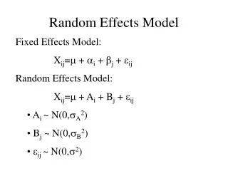
Methodological Considerations • Existing literature focussed on fixed effects modelling (and classical estimation) • By contrast, random effects model for area push and pull scores may have lower effective model dimension • Additionally, Bayesian approach assists in estimation and assessing distributional properties of push/pull indices
Properties of Push-Pull Scores • Push and pull effects may well be spatially correlated (e.g. places with high attractivity concentrated in certain regions) • Push and pull effects may be correlated with each other within areas. • Easier to model such correlation with a (Bayesian) random effects approach
Model for Migrant Flows • Consider migration flows yij from origin areas i to destination areas j (i,j=1,..n; i≠j). • Migration relatively rare in relation to origin populations Pi, but considerable variability in rates likely. • So Poisson but with overdispersion. For English migration flows in case study, mean of yij is 16.9 but standard deviation is 81. • Assume Poisson-gamma mixing (marginally negative binomial).
Negative Binomial Migration Interaction Model • yij ~ Po(ijij), ij~Ga(,) • Then integrating out ij P(yij)=kij {/(ij+)} {ij/(ij+)}yij kij= (yij+)/[(yij+1)()] >0 and log(ij) can be modelled as function of attributes of areas i and j.
Gravity Model (via NegBin Regression) • Following principle of well known gravity model, need to allow for (a) mass effects in origin & destination (b) distance decay. • Population, employment or housing stocks may measure mass effects. Here take populations Pi and Pj as mass measures. Rather than taking logPi as offset (with known parameter 1), may allow for regression effect. • So log(ij)=0+1logPi +2logPj +log(dij)
Including Accessibility • Traditional gravity model including masses and distance only insensitive to spatial structure (Fik & Mulligan, 1998). So include accessibility index Aj=rjPr/drj Large Aj values indicate alternatives in close proximity to other alternatives; low values for isolated alternatives • So log(ij)=0+1logPi +2logPj +log(dij)+log(Aj) where 1 and 2 expected to be close to 1, is negative (distance decay), typically between -0.5 and -2.
Extended Gravity Model Incorporating Random Push-Pull Effects • However, we seek summary indices of area specific push and pull indices after controlling for migration context. • Extended gravity model proposed with log(ij)=0+1logPi +2logPj +log(dij) +log(Aj)+s1i+s2j
Bivariate Random Push-Pull Effects • Bivariate push-pull effects by area si= (s1i,s2i), random with zero means over all areas. • They are spatially correlated, and also potentially correlated (+ve’ly or –ve’ly) with each other within areas.
Correlation between push-pull effects • Negative correlation within areas between push & pull scores anticipated if migration plays ‘equilibrating’ role in job markets. • In fact many studies show +ve association between in- and out-migration. Compositional hypothesis: areas with high in-migration possess large number of persons likely to move again, so increasing out-migration.
Quality of Life vs Job-Led • Declining relevance of job-led model: migration attractiveness even for working age groups increasingly related to quality of life considerations. • Counterurbanising migration to less rural areas (e.g. into South West England) may actually run counter to economic opportunities.
Prior for random push & pull effects in extended gravity model • Simple to implement bivariate spatial prior via WINBUGS using mv.car density. • Multivariate CarNormal Prior is example of Markov Random Field (Rue & Held, 2005).
WINBUGS Case Study Application • All age migrant flows yij between n=354 English Local Authorities in 2000-2001 (from 2001 UK Census). Read flow data in stacked form with intra flows (area i to area i) omitted, so have n(n-1)=124962 rows. • Three models for spatial Push-Pull effects in extended GM using NB regression • Assess fit using DIC and log of pseudo marginal likelihood (based on estimates of conditional predictive ordinates)
Models • Model 1 Independent fixed effect N(0,100) priors on each s1i ands2i. Also NormalN(0,100) priors on parameters {0,1,2,,}, and U(0,1000) prior on . • Model 2 Separate Univariate CARs on {s1i,s2i}. Priors as in model 1 except Gamma priors on spatial effect precisions 1 and 2. • Model 3 Bivariate CAR on {s1i,s2i}. Priors as in model 1 except Wishart prior on within area precision matrix .
Fit and Results • Better Fit for Model 3 with Random Effects Push-Pull Correlation Explicit in Prior • Posterior means in Model 3 (all significant) 1=0.72, 2=0.62,=-1.4,=0.066, =0.68 • Highest attractivities in model 3 concentrated in SW England, East Anglia and less urban parts of North, though some regional centres and university towns also figure. There is obvious spatial correlation when scores are mapped
High attractivity areas are mix of less urban areas which may offer higher quality of life (e.g. Cornwall, East Anglia), & areas where mobile groups (students, seasonal workers) create high migrant turnover. • Nevertheless in attractive areas attractivity index exceeds push index, so high attractivity not just a matter of flows by mobile groups but attraction of quality of life also relevant
Results High posterior correlation (0.93) between pull and push indices in model 3. Correlation between two sets of effects also 0.88 in fixed effects model 1 when correlation not incorporated a priori. Compositional hypothesis (+ve push-pull relationship due to mobile groups raising both inflows and outflows) supported. Low attractivities concentrate in Midlands & London
Age Group Models • Can apply same approach to age-specific migration, e.g. young adult migration (ages 18 to 29) or retirement migration. • Apply model 3 approach to migration by 18-29 year age group • Still have highly correlated push & pull scores (0.89) • Still have high pull scores for SW, but London also has high attractivity for this age group, esp in terms of average (push-pull)
Young adult migrant push-pull scores; correlations with area indices
Retirement Migration • Model 3 applied to migration by over 60s • Markedly high attractivity for South West, and for less urban (and lower housing cost) areas
Final Remarks • Other possible priors on random push & pull scores (e.g. mixture of structured & unstructured) • Alternative to Neg-Bin is lognormal e.g. using transform zij=log(yij+1). Distribution of errors needs to be checked – see Flowerdew & Aitken (J Reg Stud 1982) • Work by Fotheringham et al (2000) using lognormal approximation (and including Scottish areas). This shows quality of life factors & high attractivity of areas in less urban regions holds even for young adult migrants (those most likely to be ‘job-led’ migrants)