Download
1 / 99
990 likes | 1k Views
Learn about descriptive and inferential statistical methods, the importance of data context, variables, displays for different types of variables, and distributions in this comprehensive statistics overview.

E N D
Statistics BasicsAlyson Wilsonagwilso2@ncsu.eduAugust 18 and 20, 2018
Statistics Overview • There are (roughly) two categories of statistical methods. • Descriptive statistics: describe, show or summarize data in a meaningful way such that, for example, patterns might emerge from the data. • Inferential statistics: use a random sample of data taken from a population to describe and make inferences about the some property of the population. Inferential statistics are valuable when it is not convenient or possible to examine each member of an entire population. • We will also look at the idea of a model, which is a formal abstraction of data.
What’s the first rule of data analysis? LOOK AT YOUR DATA!
What are data? 17, 21, 44, 76 Test scores? Ages in a golf foursome? Uniform numbers for the football team? This is just a collection of numbers unless we have a context.
The “W’s” • A context is defined by the W’s • Who • What (and in what units) • When • Where • Why (if possible) • and How of the data. • Note: the answers to “who” and “what” are especially critical.
Nambé Ware Data In 1953, Martin Eden, a former metallurgist with Los Alamos National Laboratory, develops an eight-metal alloy that retains hot and cold temperatures for long periods of time.
Who • The Who of the data tells us the individual cases about which (or whom) we have collected data. • Individuals who answer a survey are called respondents. • People on whom we experiment are called subjectsor participants. • Animals, plants, and inanimate subjects are called experimental units. The rows of a data table correspond to the individual cases—the “who”
What The characteristics recorded about each individual are called variables. (What else are they called?) A good rule of thumb: The columns of a data table correspond to the variables—the “what”
What are some of the things that you should look for? • Types of variables • Ranges of variables • Outliers • Missing values • Summary statistics • Distribution of data Descriptive Statistics
Kinds of Variables • If a variable names categories and answers questions about how cases fall into those categories, it is called a categorical variable. • When a measured variable with units answers questions about the quantity of what is measured, we call it a quantitative or continuous variable.
Displays for Continuous Variables • Stem-and-leaf plot (stem()) • Dot plot (dotchart()) • Scatterplot (plot()) • Time-sequence plot (plot()) • Histogram (hist()) • Boxplot (boxplot()) preserve data emphasize shape
Displays for Categorical Variables • Bar chart/relative frequency bar chart • Frequency/relative frequency table • Mosaic/Marimekko chart • Pie chart be careful
Frequency Table A frequency table is a table with counts for each category. If the counts are replaced with proportions, the table is called a relative frequency table. Political Leanings Liberal 21 Moderate 23 Conservative 5 Political Leanings Liberal 0.43 Moderate 0.47 Conservative 0.10
Mosaic Plot • Survival on the Titanic. • Start with square • Proportional split along successive variables • Blue survived. • Each “tile’s” area is proportional to the counts in that cell (see Hartigan and Kleiner (1981) for original paper).
Describing Distributions • Shape • Is it symmetric? • Symmetric = roughly equal on both sides • Skewed = more values on one side • skewed left, smears out to smaller values • skewed right, smears out to larger values • Are there any outliers? • Interesting observations in data • Can impact statistical methods
Describing Distributions • Shape • How many humps (called modes)? • None = uniform • One = unimodal • Two = bimodal • Three or more = multimodal
Describing Distributions • Where is the typical value located? • Center • Median • Mean • How far apart are the values? • Spread • Range • Interquartile Range (IQR) • Standard deviation (s)
Describing Distributions • Center and Spread • Median (Center) • Range (Spread) • IQR (Spread) • Center and Spread • Mean (Center) • Standard deviation (Spread)
Boston Housing • What’s a row? • Data on census tracts in Boston from 1970 . • A census tract is a geographic region defined for the purpose of taking a census. Usually these coincide with the limits of cities, towns or other administrative areas and several tracts commonly exist within a county. • Census tracts are “Designed to be relatively homogeneous units with respect to population characteristics, economic status, and living conditions, census tracts average about 4,000 inhabitants.”
“Looking at” the Boston Housing Data CRIM Crime rate ZN % residential land zoned for lots over 0.57 acre INDUS % land occupied by nonretail business (proxy for industry) CHAS bounds Charles River NOX Nitric oxide concentration in parts per 10 million (proxy for air pollution) RM Average rooms per dwelling (proxy for spaciousness) AGE % owner-occupied units build prior to 1940 DIS Weighted distances to five Boston employment centers RAD Index of accessibility to radial highways (proxy for good location) TAX Full-value property tax rate per $10,000 PTRATIO Pupil/teacher ratio by town (proxy for school quality) B 1000(Black – 0.63)2 (Why transformed? Low-moderate hypothesized to depress prices, but high may inflate prices) LSTAT % Lower status of the population 0.5*(proportion of adults without some high-school education + proportion of male workers classified as laborers) MEDV Median value of owner-occupied homes in $1000s CAT-MEDV Median value > $30,000
“Looking at” the Boston Housing Data • Plot each variable • Calculate summary statistics • Describe the distributions and plots
Populations and Samples • Population (Big Who) • Group of people we want information from. • Generally, very large. • Impractical or prohibitively expensive to talk to everyone • Sample (Small Who) • Smaller group of people from population. • Group we get information from. • Want sample to be representative of the population • Ex: Literary Digest presidential poll in 1936.
What’s a model? A model is a simple general description of a population We’ll pick the model using different features (e.g., shape, center, spread, continuous/discrete) There is variability in our observed data: perhaps from unit-to-unit variability, perhaps because of measurement errors. What other sources cause variability in data?
Newcomb’s Data Simon Newcomb set up an experiment in 1882 to measure the speed of light. Newcomb measured the amount of time required for light to travel a distance of 7442 meters (the distance from his laboratory on the Potomac River to the Washington Monument and back). The data are recorded as deviations from 24,800 nanoseconds. (Based on the currently accepted speed of light, the “true” value is 33.)
Normal Distribution • Shape • “Bell curve” • Symmetric • Unimodal • Center (mean m) • Spread (s.d.s) • Continuous
Poisson Distribution • Unimodal • Center (mean l) • Spread (s.d. ) • Discrete (counts) Model Sample
Exponential Distribution • Center (mean l) • Spread (s.d.l) • Unimodal • Right skew • Continuous
More on Models • The class of models we are considering are called “probability distributions” • Much like data, it is useful to group these models into “discrete” and “continuous” • The models are specified with a small number of parameters
More on Models • To identify a particular model, we use its name and the parameter list • Normal(m,s2) • Poisson(l) • Exponential(l) • Some models have one parameter, some two, some three, some a vector of length k
More on Models Each model also has two associated functions: the density (continuous) or mass (discrete) function and the cumulative distribution function. The density/mass function is the function that was plotted on the previous slides (e.g., the normal “bell” curve). The cumulative distribution function is calculated from the density/mass function using integration/summation.
Definitions • A random variable is an unknown numerical quantity about which we make probability statements • A discrete random variable is one that has isolated or separated possible values (rather than a continuum of possible outcomes). • Note that there may be an infinite number of possible values • A continuous random variable is one that can be idealized as having an entire (continuous) interval of numbers as its set of possible values.
Discrete Probability Distributions A probability mass function for a discrete random variable X that can take on possible values x1, x2, . . ., is a non-negative function f(x), with f(xi) giving the probability that X takes on the value xi. • f(xi) ≥ 0 • Σ f(xi) = 1
Expected Value The mean or expected value of a discrete random variable X is E[X] =
Variance The variance of a discrete random variable X is Var[X] = = - E[X]2 The standard deviation of X is
Bernoulli • Large (infinite) population of units, interested in a variable with two values: x1 = 0, x2 = 1. A proportion p of the units have value x2 = 1. • There is an event of interest in an experiment (that we will repeat a large number of times), and it occurs with probabilityp. X = x1 = 0, if the event does not occur in the experiment, and X = x2= 1 if the event does occur. P[X = x2] = p P[X = x1] = 1 - p
Binomial Suppose that we are doing an experiment where we repeat the same “success-failure” trials n times. Assumptions • There is a constant probability of success on each trial. Call this probability p. • The repetitions are independent; knowing the outcome of any trial does not change the assessment of what would happen on another trial
Binomial Let X be the number of successes we see in the n trials. binomial(n,p) P[X = x] x = 0, 1, 2, 3, . . ., n; 0 < p < 1 E[X] = np Var[X] = np(1-p)
Poisson X counts the number of occurrences across a specified interval. Poisson(l) P[X = x] = x = 0, 1, 2, 3, . . . .; l > 0 E[X] = λ Var[X] = λ
Cumulative Distribution Function Cumulative distribution function (cdf): F(x) for the discrete random variable X is defined as the probability that X is less than or equal to x F(x) = P[X ≤ x] =
Continuous Probability Distributions Probability density function f(x) ≥ 0 The intuition that we used for discrete random variables that the density function is the probability that X = x breaks down for continuous random variables. Why?
Continuous Probability Distributions Instead we can think about either the cumulative distribution function or about the probability that X takes on a value in some interval (a,b)
Expected Value The mean or expected value of a continuous random variable X is E[X] = E[g(X)] =
Variance The variance of a discrete random variable X is Var[X] = = - E[X]2 = E[X2] – E[X]2 The standard deviation of X is
Median The value x0 such that
Normal Distribution • Normal(m,s2) • Mean m • s.d.s
Exponential Distribution • Mean l • s.d.l • P(X > t + s | X > s) = P(X > t)