Download
1 / 66
660 likes | 855 Views
Roy Chantrell Physics Department, York University. Atomistic modelling 1: Basic approach and pump-probe calculations. Thanks to. Natalia Kazantseva, Richard Evans, Tom Ostler, Joe Barker, Physics Department University of York Denise Hinzke, Uli Nowak,

E N D
Roy Chantrell Physics Department, York University Atomistic modelling 1: Basic approach and pump-probe calculations
Thanks to Natalia Kazantseva, Richard Evans, Tom Ostler, Joe Barker, Physics Department University of York Denise Hinzke, Uli Nowak, Physics Department University of Konstanz Felipe Garcia-Sanchez, Unai Atxitia, Oksana Chubykalo-Fesenko, ICMM, Madrid Oleg Mryasov, Adnan Rebei, Pierre Asselin, Julius Hohlfeld, Ganping Ju, Seagate Research, Pittsburgh Dmitry Garanin, City University of New York Th Rasing, A Kirilyuk, A Kimel, IMM, Radboud University Nijmegen, NL
Summary • Introduction – high anisotropy materials and magnetic recording • The need for atomistic simulations • Static properties – Ising model and MC simulations • Atomistic simulations • Model development • Langevin Dynamics and Monte Carlo methods • Magnetisation reversal • Applications • Pump-Probe processes • Opto-magnetic reversal • Atomistic model of Heat Assisted Magnetic Recording (HAMR)
a Inductive GMR Read Write Element Sensor D* sj µ a d W D*= W 8-10 nm d N N S S N S S N N S N S N S B Recording Medium Media Noise Limitations in Magnetic Recording SNR ~ 10×log (B/ sj) Need sj/B<10% • Transition position jitter sj limits media noise performance! • Key factors are cluster size D* and transition width a. • Reducing the grain size runs into the so-called superparamagnetic limit – information becomes thermally unstable
Superparamagnetism • The relaxation time of a grain is given by the Arrhenius-Neel law • where f0 = 109s-1. and E is the energy barrier • This leads to a critical energy barrier for superparamagnetic (SPM) behaviour • where tm is the ‘measurement time’ • Grains with E < Ec exhibit thermal equilibrium (SPM) behaviour - no hysteresis
Minimal Stable Grain Size (cubic grains) • Time • Temperature • Anisotropy today future Write Field is limited by BS (2.4T today!)of Recording Head H0=aHK-NMS D. Weller and A. Moser, IEEE Trans. Magn.35, 4423(1999)
Bit Patterned MediaLithography vs Self Organization Lithographically Defined FePt SOMA media • Major obstacle is finding low cost means of making media. • At 1 Tbpsi, assuming a square bit cell and equal lines and spaces, 12.5 nm lithography would be required. • Semiconductor Industry Association roadmap does not provide such linewidths within the next decade. • 6.3+/-0.3 nm FePt particles • sDiameter@0.05 S. Sun, Ch. Murray, D. Weller, L. Folks, A. Moser, Science 287, 1989 (2000).
Modelling magnetic properties:The need for atomistic/multiscale approaches • Standard approach (Micromagnetics) is based on a continuum formalism which calculates the magnetostatic field exactly but which is forced to introduce an approximation to the exchange valid only for long-wavelength magnetisation fluctuations. • Thermal effects can be introduced, but the limitation of long-wavelength fluctuations means that micromagnetics cannot reproduce phase transitions. • The atomistic approach developed here is based on the construction of a physically reasonable classical spin Hamiltonian based on ab-initio information.
Micromagnetic exchange • The exchange energy is essentially short ranged and involves a summation of the nearest neighbours. Assuming a slowly spatially varying magnetisation the exchange energy can be written Eexch = Wedv, with We = A(m)2 (m)2 = (mx)2 + (my)2 + (mz)2 • The material constant A = JS2/a for a simple cubic lattice with lattice constant a. A includes all the atomic level interactions within the micromagnetic formalism.
Relation to ab-initio calculations and micromagnetics • Ab-initio calculations are carried out at the electronic level. • Number of atoms is strictly limited, also zero temperature formalism. • Atomistic calculations take averaged quantities for important parameters (spin, anisotropy, exchange, etc) and allow to work with 106 to 108 spins. Phase transitions are also allowed. • Micromagnetics does a further average over hundreds of spins (continuum approximation) • Atomistic calculations form a bridge • Lecture 1: concentrates on the link to ab-intio calculations – development of a classical spin Hamiltonian for FePt from ab-initio calculations and comparison with experiment. • Lecture 2: Development of multi-scale calculations- link to micromagnetics via the Landau-Lifshitz-Bloch (LLB equation).
Calculation of equilibrium properties • Description of the properties of a system in thermal equilibrium is based on the calculation of the partition function Z given by where S is representative of the spin system • If we can calculate Z it is easy to calculate thermal average properties of some quantity A(S) as follows Where p(S) is the probability of a given spin-state
Monte-Carlo method • It would be possible in principle to do a numerical integration to calculate <A>. • However, this is very inefficient since p(S) is strongly peaked close to equilibrium. • A better way is to use ‘importance sampling’, invented by Metropolis et al
Importance sampling • We define a transition probability between states such that the ‘detailed balance condition is’ obeyed • The physics can be understood given that p(S)=Z-1exp(-H(S)/kBT), ie p(S) does not change with time at equilibrium.
Metropolis algorithm • For a given state choose a spin i (randomly or sequentially), change the direction of the spin, and calculate the energy change DE. • If DE < 0, allow the spin to remain in the new state. If DE > 0, choose a uniformly distributed random number r [0; 1]. if r < exp(-DE/kBT) allow the spin to remain in the new state, otherwise the spin reverts to its original state. • Iterate to equilibrium • Thermal averages reduce to an unweighted summation over a number (N) of MC moves, eg for the magnetisation
Summary • Thermodynamic properties of magnetic materials studied using Ising model • Analytical and mean-field model • MC approach for atomistic calculations agrees well with analytical mode (Onsager) • In the following we introduce a dynamic approach and apply this to ultrafast laser processes
Atomistic model of dynamic properties • Uses the Heisenberg form of exchange • Spin magnitudes and J values can be obtained from ab-initio calculations. • We also have to deal with the magnetostatic term. • 3 lengthscales – electronic, atomic and micromagnetic – Multiscale modelling.
Ab-initio information (spin, exchange, etc) Dynamic response solved using Langevin Dynamics (LLG + random thermal field term) Classical spin Hamiltonian Magnetostatics Model outline Static (equilibrium) processes can be calculated using Monte-Carlo Methods
Dynamic behaviour • Dynamic behaviour of the magnetisation is based on the Landau-Lifshitz equation Where g0 is the gyromagnetic ratio and a is a damping constant
Langevin Dynamics • Based on the Landau-Lifshitz-Gilbert equations with an additional stochastic field term h(t). • From the Fluctuation-Dissipation theorem, the thermal field must must have the statistical properties • From which the random term at each timestep can be determined. • h(t) is added to the local field at each timestep.
M vs T; static (MC) and dynamic calculations • Dynamic values are calculated using Langevin Dynamics for a heating rate of 300K/ns. • Essentially the same as MC values. • Fast relaxation of the magnetisation (see later)
How to link atomistic and ab-initio calculations? • Needs to be done on a case-by-case basis • In the following we consider the case of FePt, which is especially interesting. • First we consider the ab-initio calculations and their representation in terms of a classical spin Hamiltonian. • The model is then applied to calculations of the static and dynamic properties of FePt.
Ab-initio/atomistic model of FePt • Anisotropy on Pt sites • Pt moment induced by the Fe • Treating Pt moment as independent degrees of freedom gives incorrect result (Low Tc and ‘soft’ Pt layers) • New Hamiltonian replaces Pt moment with moment proportional to exchange field. Exchange values from ab-initio calcuations. • Long-ranged exchange fields included in a FFT calculation of magnetostatic effects • Langevin Dynamics used to look at dynamic magnetisation reversal • Calculations of • Relaxation times • Magnetisation vs T
Disorder to Order Transformation 50% Fe/50% Pt After Anneal Fe As Deposited Pt b b b b c a Anneal a a a Ordered L10 (ex. FePt) FCC disordered alloy Small cubic Anisotropy ra=fraction of a sites occupied by correct atom xA=atom fraction of A yb=fraction of b sites Degree of Chemical Order = S
FePt exchange • Exchange coupling is long ranged in FePt
FePt Hamiltonian Exchange: Fe/Fe Fe/Pt Pt/Pt Anisotropy Zeeman Convention: Fe sites i,j Pt sites k,l
Localisation (ab-initio calculations) To good approximation the Pt moment is found numerically to be Exchange field from the Fe
Thus we take the FePt moment to be given by With Substitution for the Pt moments leads to a Hamiltonian dependent only on the Fe moments;
With new effective interactions Single ion anisotropy 2-ion anisotropy (new term) And moment .
All quantities can be determined from ab-initio calculations • 2-ion term (resulting from the delocalised Pt degrees of freedom) is dominant
New Hamiltonian replaces Pt moment with moment proportional to exchange field from Fe. Gives a 2 ion contribution to anisotropy Exchange and K(T=0) values from ab-initio calculations. Long-ranged exchange fields included in a FFT calculation of magnetostatic effects Langevin Dynamics or Monte-Carlo approaches Can calculate M vs T K vs T Dynamic properties Good fit to experimental data (Theile and Okamoto) First explanation of origin of experimental power law – results from 2 ion anisotropy Anisotropy of FePt nanoparticles
Model of magnetic interactions for ordered 3d-5d alloys: Temp. dependence of equilibrium properties. Reasonable estimate of Tc (no fitting parameters)
Unusual properties of FePt 1: Domain Wall directionality Atomic scale model calculations of the equilibrium domain wall structure
Unusual properties of FePt 2: Elliptical and linear Domain Walls • Circular (normal Bloch wall); Mtot is orientationally invariant • Elliptical; Mtot decreases in the anisotropy hard direction • Linear; x and y components vanish
Walls are elliptical at non-zero temperatures • Linear walls occur close to Tc above a critical temperature which departs further from Tc with increasing K • Analogue (see later) is linear magnetisation reversal – important new mechanism for ultrafast dynamics.
Ultrafast Laser induced magnetisation dynamics • The response of the magnetisation to femtosecond laser pulses is an important current area of solid state physics • Also important for applications such as Heat Assisted Magnetic Recording (HAMR) • Here we show that ultrafast processes cannot be simulated with micromagnetics. • An atomistic model is used to investigate the physics of ultrafast reversal.
Pump-probe experiment • Apply a heat pulse to the material using a high energy fs laser. • Response of the magnetisation is measured using MOKE • Low pump fluence – all optical FMR • High pump fluence – material can be demagnetised. • In our model we assume that the laser heats the conduction electrons, which then transfer energy into the spin system and lattice. • Leads to a ‘2-temperature’ model for the temperature of the conduction electron and lattice
Atomistic model • Uses the Heisenberg form of exchange • Dynamics governed by the Landau-Lifshitz-Gilbert (LLG) equation. • Random field term introduces the temperature (Langevin Dynamics). • Variance of the random field determined by the electron temperature Tel.
l l l Pump-probe simulations – continuous thin film • Rapid disappearance of the magnetisation • Reduction depends on l
Ultrafast demagnetisation • Experiments on Ni (Beaurepaire et al PRL 76 4250 (1996) • Calculations for peak temperature of 375K • Normalised M and T. During demagnetisation M essentially follows T